Using Convpaint & Python - Introduction#
Here, we show you the basics of using Convpaint programmatically with Python. Concretely, we will present 3 ways to use the Convpaint GUI and/or API:
a) Using Convpaint as a napari plugin (GUI), only accessing and processing the results programmatically afterwards
b) Training a Convpaint model in the GUI, then using it programmatically (API) for segmenting new images
c) Using the Convpaint API from end to end, without the GUI
When you intend to use Convpaint programmatically, it is important to understand the Convpaint API and its main concepts.
All the information you need can be found in the docs, notably the following resources:
Imports#
import napari
import matplotlib.pyplot as plt
import os
from napari_convpaint import ConvpaintModel
import numpy as np
a) Use Convpaint entirely in Napari - only access results via API#
Open a napari viewer from within Python to make its data accessible from there (this might take a while the first time, as napari will load all its plugins).
viewer = napari.Viewer()
In Napari:
Open the Convpaint Plugin (this might take a while the first time, as Convpaint will load its models)
Use Convpaint as usual to train a model and segment an image (e.g. with the “Cells 2D” sample image)
Access the results as illustrated below
seg = viewer.layers['segmentation'].data
img = viewer.layers['Cells 2D'].data
Display the results to verify it worked.
plt.imshow(img)
plt.imshow(seg, alpha=0.5)
plt.axis('off')
plt.show()
From here, we could do post-processing and further analysis using packages like skimage, pandas and seaborn.
See the examples section for some inspiration.
b) Train a model in the GUI, then use it programmatically (API)#
Repeat the steps above until training a model in the GUI, but then save the model as pickle file (in this example BCSS_default_model.pkl).
viewer2 = napari.Viewer()
Then, you can load the model in Python. To check what model we loaded, we can print its parameters.
cpm = ConvpaintModel(model_path="BCSS_default_model.pkl")

for p in cpm.get_params().items():
    print(p)
('classifier', 'CatBoost')
('channel_mode', 'rgb')
('normalize', 3)
('image_downsample', 1)
('seg_smoothening', 1)
('tile_annotations', True)
('tile_image', False)
('use_dask', False)
('unpatch_order', 1)
('fe_name', 'vgg16')
('fe_use_gpu', False)
('fe_layers', ['features.0 Conv2d(3, 64, kernel_size=(3, 3), stride=(1, 1), padding=(1, 1))'])
('fe_scalings', [1, 2, 4])
('fe_order', 0)
('fe_use_min_features', False)
('clf_iterations', 100)
('clf_learning_rate', 0.1)
('clf_depth', 5)
('clf_use_gpu', None)
And now we can use it in Python on new images.
Note that Convpaint could also segment a batch of images at once (see below), but since here we loop over them for loading anyway, we just segment them one by one.
Note that this happens automatically when using Convpaint in Napari, but needs to be done manually when using the API.
image_folder = "BCSS_examples/BCSS_windows"

imgs = []
segs = []
for i, file in enumerate(os.listdir(image_folder)):
    if not file.endswith(".png"):
        continue
    img = plt.imread(image_folder + "/" + file)
    print(f"Processing image {i+1}: {img.shape}")
    img = np.moveaxis(img, -1, 0)  # move channel last to channel first
    print(f"Reshaped image:     {img.shape}")

    seg = cpm.segment(img) # HERE WE SEGMENT THE IMAGES

    imgs.append(img)
    segs.append(seg)
Processing image 1: (1326, 1297, 3)
Reshaped image:     (3, 1326, 1297)
Processing image 2: (1326, 1297, 3)
Reshaped image:     (3, 1326, 1297)
Processing image 3: (1326, 1297, 3)
Reshaped image:     (3, 1326, 1297)
Processing image 4: (1326, 1297, 3)
Reshaped image:     (3, 1326, 1297)
And we can display the results.
assert len(imgs) == len(segs) # sanity check that we have the same number of images and segmentations

fig, axs = plt.subplots(2, len(imgs), figsize=(4*len(imgs), 8))
for i, img in enumerate(imgs):
    axs[0, i].imshow(np.moveaxis(img, 0, -1)) # move channel first back to channel last for visualization
    axs[0, i].set_title(f"Input Image {i+1}")
    axs[1, i].imshow(segs[i])
    axs[1, i].set_title(f"Segmentation {i+1}")
    for ax in axs[:, i]:
        ax.axis('off')
plt.show()

c) Use Convpaint entirely in Python#
1. Create and set up model#
Create a ConvpaintModel instance. See the separate page for more options for initialization.
cpm2 = ConvpaintModel() # create a default model (without a trained classifier)
Change parameters, just like in the GUI. Again, refer to the separate page describing all parameters.
# First get an overview of the available parameters and their default values
for p in cpm2.get_params().items():
    print(p)
('classifier', None)
('channel_mode', 'single')
('normalize', 2)
('image_downsample', 1)
('seg_smoothening', 1)
('tile_annotations', True)
('tile_image', False)
('use_dask', False)
('unpatch_order', 1)
('fe_name', 'vgg16')
('fe_use_gpu', False)
('fe_layers', ['features.0 Conv2d(3, 64, kernel_size=(3, 3), stride=(1, 1), padding=(1, 1))'])
('fe_scalings', [1, 2, 4])
('fe_order', 0)
('fe_use_min_features', False)
('clf_iterations', 100)
('clf_learning_rate', 0.1)
('clf_depth', 5)
('clf_use_gpu', None)
# Now set some parameters to non-default values
cpm2.set_params(channel_mode="multi", normalize=3, seg_smoothening=2)
2. Train the model#
Now, we first need to train the model.
For this, we need images and corresponding annotations. Remember to move the channels to the first dimension if needed.
NOTE: To read annotations, we here use skimage.io.imread instead of plt.imread, as the latter will rescale the values to [0, 1], which we do not want for annotations. You could also manually rescale the values back to integers, but using skimage.io.imread is easier.
image_folder = "cellpose_examples"

img0 = plt.imread(image_folder + "/" + "000_img.png")

import skimage
annot0 = skimage.io.imread(image_folder + "/" + "000_scribbles_all_01000_w1_run07_annot.png")

print(f"Image shape: {img0.shape}, Annotations shape: {annot0.shape}")
img0 = np.moveaxis(img0, -1, 0)  # move channel last to channel first
print(f"Reshaped image: {img0.shape}")
Image shape: (383, 512, 3), Annotation shape: (383, 512)
Reshaped image: (3, 383, 512)
print(np.unique(annot0)) # check unique labels in the annotations
print(f"Num annotated pixels: 1 = {(annot0 == 1).sum()}, 2 = {(annot0 == 2).sum()}") # check number of pixels per label
[0 1 2]
Num annotated pixels: 1 = 983, 2 = 940
clf = cpm2.train(img0, annot0) # HERE WE TRAIN THE MODEL
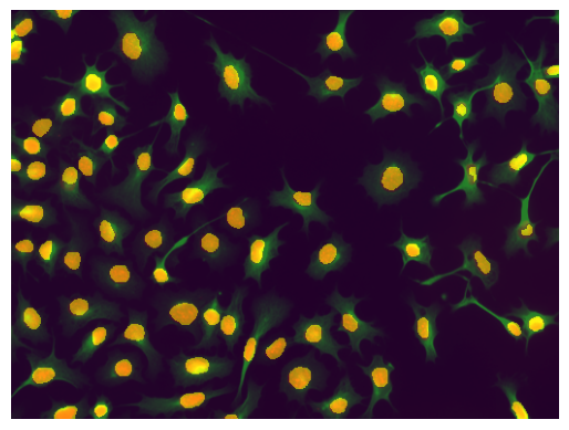
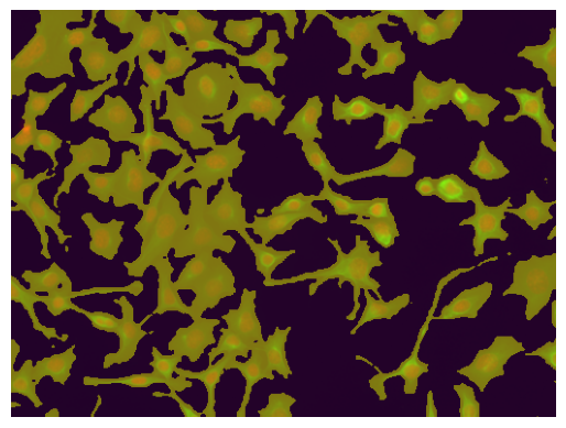
3. Segment new images#
img1 = plt.imread(image_folder + "/" + "001_img.png")
img1 = np.moveaxis(img1, -1, 0)  # move channel last to channel first


seg = cpm2.segment(img1)

plt.imshow(np.moveaxis(img1, 0, -1)) # move channel first back to channel last for visualization
plt.imshow(seg, alpha=0.5)
plt.axis('off')
plt.show()
FE model is designed for imagenet normalization, but image is not declared as 'rgb' (parameter channel_mode). Using default normalization instead.
Optional: Train on multiple images#
We can also train on multiple images and annotations at once by passing lists of arrays.
img_names =["000_img.png", "001_img.png"]
annot_names =["000_scribbles_all_01000_w1_run07_annot.png", "001_scribbles_all_01000_w1_run07_annot.png"]

imgs = [plt.imread(image_folder + "/" + name) for name in img_names]
imgs = [np.moveaxis(img, -1, 0) for img in imgs]  # move channel last to channel first

annots = [skimage.io.imread(image_folder + "/" + name) for name in annot_names]
cpm3 = ConvpaintModel(fe_name="vgg16", channel_mode="multi", normalize=3, seg_smoothening=2)
clf = cpm3.train(imgs, annots) # HERE WE TRAIN ON MULTIPLE IMAGES
FE model is designed for imagenet normalization, but image is not declared as 'rgb' (parameter channel_mode). Using default normalization instead.
FE model is designed for imagenet normalization, but image is not declared as 'rgb' (parameter channel_mode). Using default normalization instead.
0:	learn: 0.5355210	total: 11ms	remaining: 1.09s
1:	learn: 0.4268868	total: 22.5ms	remaining: 1.1s
2:	learn: 0.3455982	total: 31.7ms	remaining: 1.02s
3:	learn: 0.2939234	total: 40.7ms	remaining: 977ms
4:	learn: 0.2505869	total: 49.5ms	remaining: 941ms
5:	learn: 0.2164440	total: 58.2ms	remaining: 913ms
6:	learn: 0.1882357	total: 68.1ms	remaining: 905ms
7:	learn: 0.1697273	total: 76.2ms	remaining: 876ms
8:	learn: 0.1547895	total: 85.3ms	remaining: 863ms
9:	learn: 0.1432902	total: 93.8ms	remaining: 844ms
10:	learn: 0.1303033	total: 103ms	remaining: 833ms
11:	learn: 0.1214221	total: 112ms	remaining: 819ms
12:	learn: 0.1140107	total: 120ms	remaining: 805ms
13:	learn: 0.1076304	total: 129ms	remaining: 791ms
14:	learn: 0.1019194	total: 137ms	remaining: 778ms
15:	learn: 0.0957654	total: 146ms	remaining: 768ms
16:	learn: 0.0911031	total: 154ms	remaining: 754ms
17:	learn: 0.0881742	total: 163ms	remaining: 741ms
18:	learn: 0.0824428	total: 171ms	remaining: 728ms
19:	learn: 0.0804849	total: 179ms	remaining: 717ms
20:	learn: 0.0770931	total: 188ms	remaining: 708ms
21:	learn: 0.0737597	total: 197ms	remaining: 698ms
22:	learn: 0.0707649	total: 205ms	remaining: 685ms
23:	learn: 0.0697660	total: 213ms	remaining: 676ms
24:	learn: 0.0685446	total: 221ms	remaining: 664ms
25:	learn: 0.0661318	total: 230ms	remaining: 655ms
26:	learn: 0.0630170	total: 238ms	remaining: 644ms
27:	learn: 0.0606994	total: 248ms	remaining: 637ms
28:	learn: 0.0583657	total: 258ms	remaining: 631ms
29:	learn: 0.0567362	total: 267ms	remaining: 623ms
30:	learn: 0.0553210	total: 275ms	remaining: 613ms
31:	learn: 0.0535005	total: 285ms	remaining: 606ms
32:	learn: 0.0522592	total: 294ms	remaining: 596ms
33:	learn: 0.0504603	total: 302ms	remaining: 586ms
34:	learn: 0.0483266	total: 311ms	remaining: 578ms
35:	learn: 0.0473808	total: 320ms	remaining: 568ms
36:	learn: 0.0459419	total: 329ms	remaining: 560ms
37:	learn: 0.0446647	total: 337ms	remaining: 549ms
38:	learn: 0.0434622	total: 346ms	remaining: 541ms
39:	learn: 0.0427531	total: 354ms	remaining: 531ms
40:	learn: 0.0416013	total: 363ms	remaining: 523ms
41:	learn: 0.0408790	total: 372ms	remaining: 513ms
42:	learn: 0.0397381	total: 380ms	remaining: 504ms
43:	learn: 0.0394235	total: 388ms	remaining: 494ms
44:	learn: 0.0387579	total: 397ms	remaining: 485ms
45:	learn: 0.0381533	total: 405ms	remaining: 475ms
46:	learn: 0.0367724	total: 413ms	remaining: 466ms
47:	learn: 0.0364169	total: 421ms	remaining: 456ms
48:	learn: 0.0358266	total: 430ms	remaining: 447ms
49:	learn: 0.0353280	total: 438ms	remaining: 438ms
50:	learn: 0.0347162	total: 447ms	remaining: 429ms
51:	learn: 0.0342091	total: 455ms	remaining: 420ms
52:	learn: 0.0332666	total: 465ms	remaining: 412ms
53:	learn: 0.0325733	total: 474ms	remaining: 404ms
54:	learn: 0.0318575	total: 483ms	remaining: 395ms
55:	learn: 0.0306957	total: 492ms	remaining: 387ms
56:	learn: 0.0301558	total: 501ms	remaining: 378ms
57:	learn: 0.0294657	total: 510ms	remaining: 369ms
58:	learn: 0.0291038	total: 518ms	remaining: 360ms
59:	learn: 0.0289394	total: 526ms	remaining: 351ms
60:	learn: 0.0285454	total: 534ms	remaining: 341ms
61:	learn: 0.0277977	total: 543ms	remaining: 333ms
62:	learn: 0.0271670	total: 551ms	remaining: 324ms
63:	learn: 0.0269450	total: 560ms	remaining: 315ms
64:	learn: 0.0261949	total: 568ms	remaining: 306ms
65:	learn: 0.0257261	total: 577ms	remaining: 297ms
66:	learn: 0.0252887	total: 586ms	remaining: 289ms
67:	learn: 0.0246148	total: 596ms	remaining: 280ms
68:	learn: 0.0244843	total: 604ms	remaining: 271ms
69:	learn: 0.0243184	total: 613ms	remaining: 263ms
70:	learn: 0.0241393	total: 621ms	remaining: 254ms
71:	learn: 0.0230771	total: 629ms	remaining: 245ms
72:	learn: 0.0227372	total: 638ms	remaining: 236ms
73:	learn: 0.0220487	total: 648ms	remaining: 228ms
74:	learn: 0.0218510	total: 656ms	remaining: 219ms
75:	learn: 0.0217699	total: 665ms	remaining: 210ms
76:	learn: 0.0211904	total: 674ms	remaining: 201ms
77:	learn: 0.0209936	total: 683ms	remaining: 193ms
78:	learn: 0.0205381	total: 692ms	remaining: 184ms
79:	learn: 0.0203644	total: 700ms	remaining: 175ms
80:	learn: 0.0202157	total: 709ms	remaining: 166ms
81:	learn: 0.0199253	total: 717ms	remaining: 157ms
82:	learn: 0.0197427	total: 726ms	remaining: 149ms
83:	learn: 0.0196567	total: 734ms	remaining: 140ms
84:	learn: 0.0193742	total: 742ms	remaining: 131ms
85:	learn: 0.0191949	total: 750ms	remaining: 122ms
86:	learn: 0.0189064	total: 760ms	remaining: 113ms
87:	learn: 0.0187050	total: 768ms	remaining: 105ms
88:	learn: 0.0182926	total: 777ms	remaining: 96ms
89:	learn: 0.0180987	total: 785ms	remaining: 87.2ms
90:	learn: 0.0179848	total: 793ms	remaining: 78.5ms
91:	learn: 0.0177471	total: 801ms	remaining: 69.7ms
92:	learn: 0.0173027	total: 810ms	remaining: 61ms
93:	learn: 0.0171361	total: 818ms	remaining: 52.2ms
94:	learn: 0.0168196	total: 827ms	remaining: 43.5ms
95:	learn: 0.0166168	total: 835ms	remaining: 34.8ms
96:	learn: 0.0163895	total: 844ms	remaining: 26.1ms
97:	learn: 0.0160646	total: 852ms	remaining: 17.4ms
98:	learn: 0.0158913	total: 861ms	remaining: 8.69ms
99:	learn: 0.0155655	total: 869ms	remaining: 0us
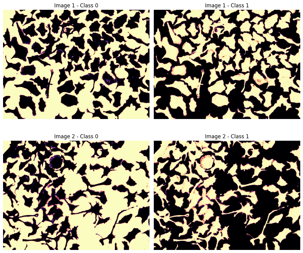
Optional: Predict probabilities, and predict multiple files#
And we can segment - or predict separate class probability maps - on a list of images as well.
probas = cpm3.predict_probas(imgs) # HERE WE PREDICT PROBABILITIES

num_imgs = len(probas)
num_classes = probas[0].shape[0]

print(f"Number of images: {num_imgs} | Number of classes: {num_classes}")
FE model is designed for imagenet normalization, but image is not declared as 'rgb' (parameter channel_mode). Using default normalization instead.
FE model is designed for imagenet normalization, but image is not declared as 'rgb' (parameter channel_mode). Using default normalization instead.
Number of images: 2 | Number of classes: 2
fig, ax = plt.subplots(nrows=num_imgs, ncols=num_classes, figsize=(10, 9))

for i, proba_im in enumerate(probas):
    for cl in range(num_classes):
        ax[i, cl].imshow(proba_im[cl], cmap='magma')
        ax[i, cl].set_title(f"Image {i+1} - Class {cl}")
        ax[i, cl].axis('off')
plt.tight_layout()
plt.show()