Detecting calcium signaling waves in timelapse movies#
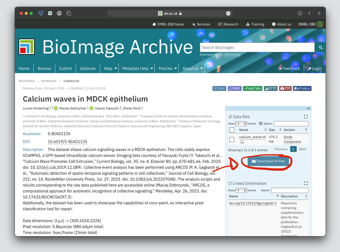
This notebook demonstrates the workflow for detecting calcium signalling waves in microscopy images using ARCOS, a tool to detect spatio-temporal signaling patterns. The data was originally acquired by Takeuchi Y. et al. (2023) and is available from the bioimage archive under accession nymber S-BIAD1135.
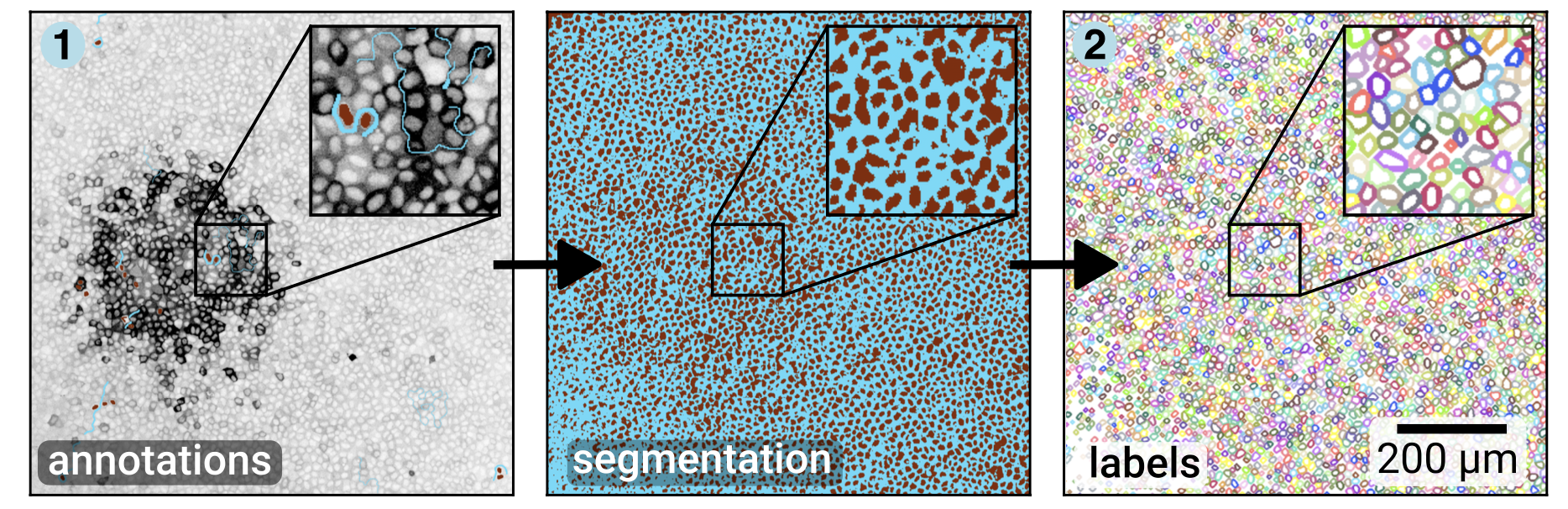
The main steps are to segment the cells with Convpaint, then process the labels to get a ring-like mask for every cell:
Then we use ARCOS for automatically detecting collective signalling events:
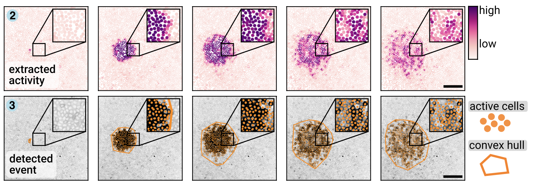
Here is a movie of the output of this script. Active cells are marked with a black dot. Collective events are outlined in color, and cells that are active and belong to the collective event are marked with a colored dot.
Before we start, make sure you have the following python packages installed:
convpaintfor segmenting the cells from the backgrounddevbio-naparilarge collection of napari plugins for bioimage analysis (we mostly need napari-assistant for post-processing the labels)btrackto track cells over timearcos-guito detect collective event
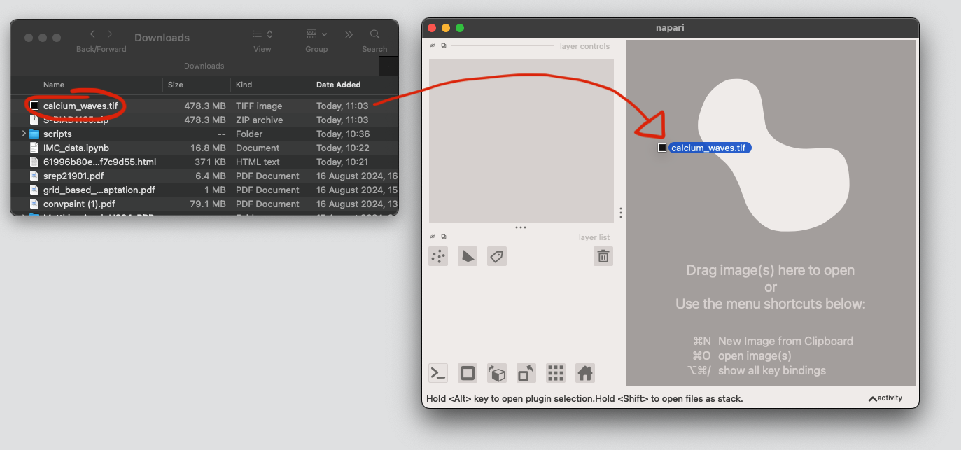
Download the data, drag-and-drop it to open in Napari#
Download the file calcium_waves.tif and unzip.
Next, open napari:
import napari
import numpy as np

viewer = napari.Viewer()
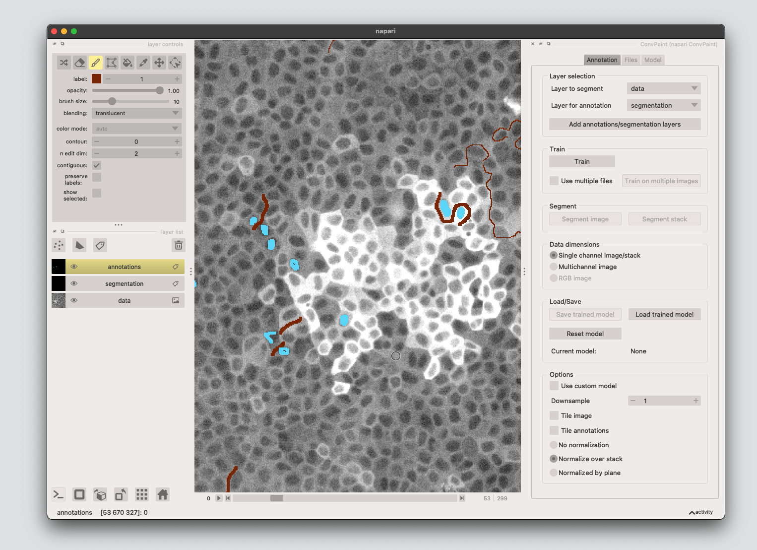
Segment the cells using conv-paint#
Drag-and-drop the .tif file to open it in napari.
Open the Convpaint plugin and start adding annotations. To reproduce our results, you can also load the annotations.npz file.
# save your own annotations:
# np.savez_compressed('../sample_data/calcium_waves_workflow/annotations.npz', a=annotations)

# load pre-made annotations (frame 53 is annotated)
annotations = np.load('../sample_data/calcium_waves_workflow/annotations.npz')['a']
viewer.add_labels(annotations, name='annotations')
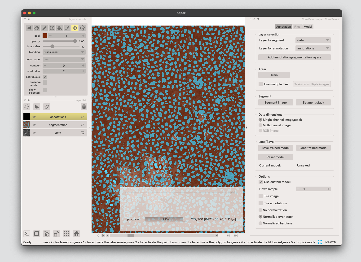
Train the classifier, check segmentation results, segment whole stack#
For this workflow, using VGG16 single-layer and input scalings 1-2-4 works well.
If you are happy with the segmentation results, click Segment stack.
You can store/load segmentation results with the following code or using the napari GUI.
# save your segmentation results
# segmentation = viewer.layers['segmentation'].data
# np.savez_compressed('../sample_data/calcium_waves_workflow/segmentation.npz', a=segmentation)

# load previous segmentation results
segmentation = np.load('../sample_data/calcium_waves_workflow/segmentation.npz')['a']
viewer.add_labels(segmentation, name='segmentation')
Post-process the labels and detect collective signalling#
Use the napari-assistant plugin for:
Convert from 3D to 2D+t format
Voronoi-otsu labelling (convert semantic to instance segmentation)
Expand the labels
Only keep the edges of the labels, creating a labeled ring for all the cells
Convert to the right data format and save
After that we will:
use the
Btracknapari plugin to track the cellsget the calcium activity of all the cells using
napari-skimage-regionpropsDetect the collective events using
ARCOS
0. Convert data format#
Convert the data from 3D to 2D timelapse format, so that it conforms with napar-assistant convention. This also enables working with on-the-fly processing - only the currently viewed frame is being processed, enabling to quickly try out different parameters. More info can be found in the napari-time-slicer github repo.
To do this, select Utilities >> Convert 3D stack to 2D timelapse (time-slicer), select the data layer containing your segmentation, then click Run. Also convert the raw calcium imaging data. You can then delete the old layers.
1. Voronoi-Otsu labelling#
From the menu choose: Plugins >> clEsperanto >> Label. You can test different Sigma values, but the default values work well here.

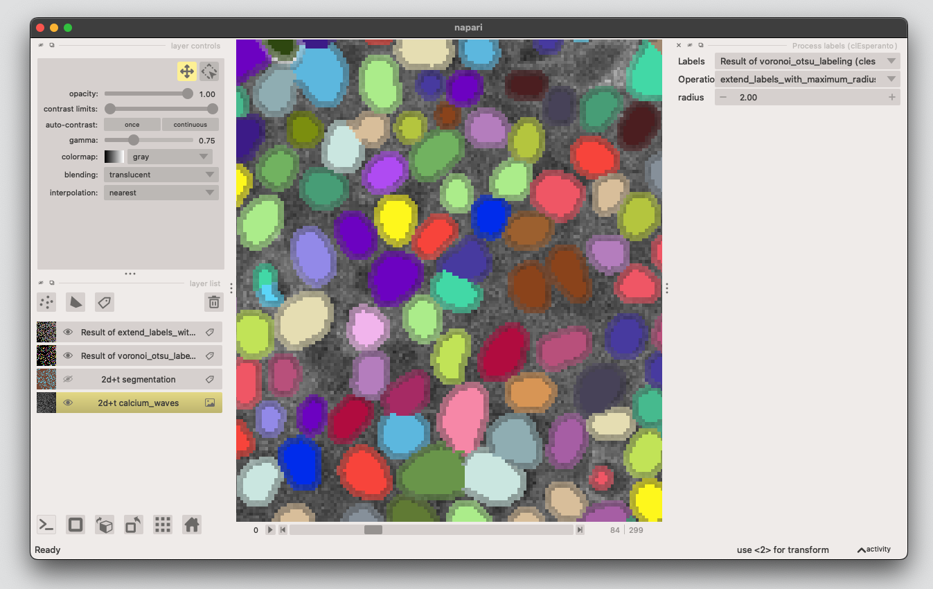
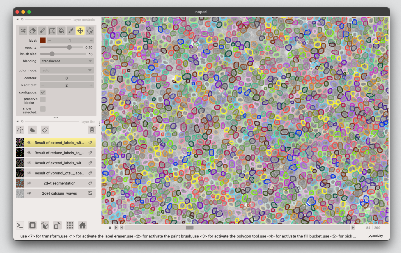
2. Expand the labels#
Open the napari-assistant, choose Process labels, then select
extend_labels_with_maximum_radius. This will create a new labels layer where the original labels are expanded by 2 px.
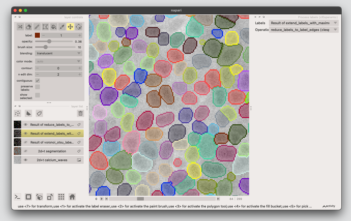
3. Create cytosolic ring#
3.1: From the napari-assistant, choose Process labels, then select
reduce_labels_to_labels_edges.
3.2: Expand the edge-labels as again like we did in the step above (choose Process labels, then select
extend_labels_with_maximum_radius)
4. Apply the processing to the whole stack#
At the moment the processing is still applied lazily to the frames on the demand. In this step we actually run in on all the frames.
Select Utilities >> Convert on-the-fly processesed timelapse to 4D stack (time-slicer). Select the layer with the latest processing and click Run.
You can rename the converted layer to e.g. edges and delete the layers with the intermediate processing steps. This is also a good timepoint to save the progress.
# save the processing results
# edges = viewer.layers['edges'].data
# np.savez_compressed('../sample_data/calcium_waves_workflow/edges.npz', a=edges)

# load the segmentation results
edges = np.load('../sample_data/calcium_waves_workflow/edges.npz')['a']
edges = np.squeeze(edges)
viewer.add_labels(edges, name='edges')
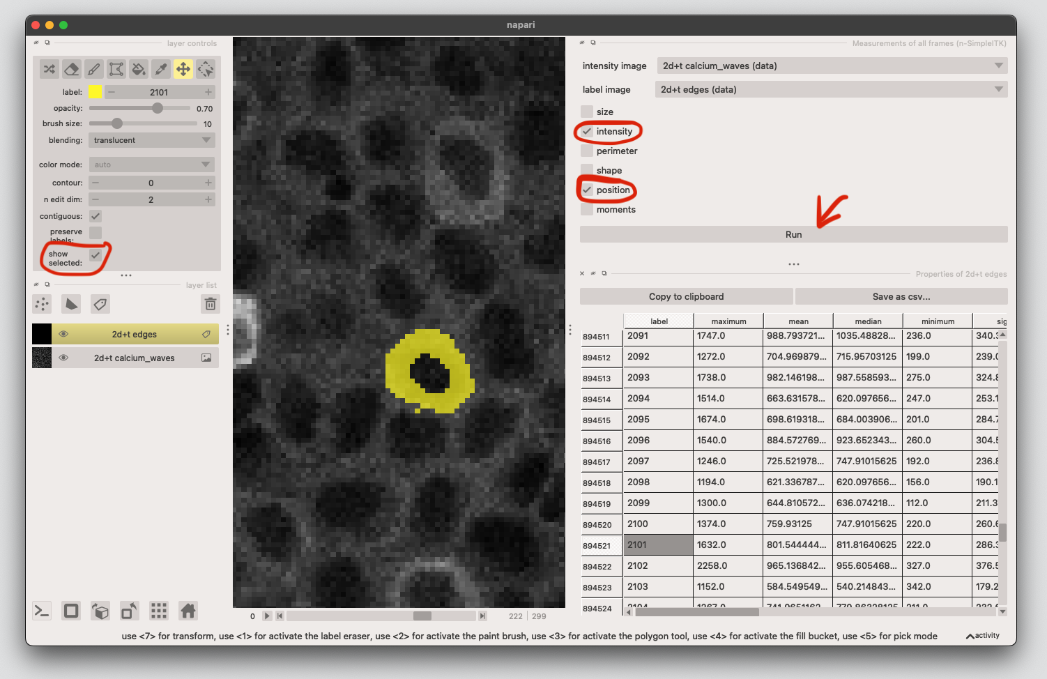
5. Get the calcium signal for each cell at each timepoint#
Extract region properties for each frame using. Select Measurements of all frames (n-SimpleITK) from the menu, select the calcium data as image and the edges as labels (make sure both are in 2D+t format).
We need the intensity and position information, tick these then click on run.
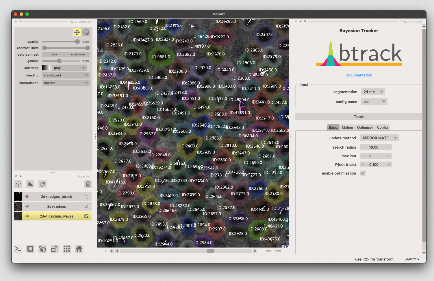
6. Track the cells using the Btrack plugin#
Next we link the edge-masks from frame to frame. Change the parameters to
update method:
APPROXIMATEsearch radius:
10max lost:
5
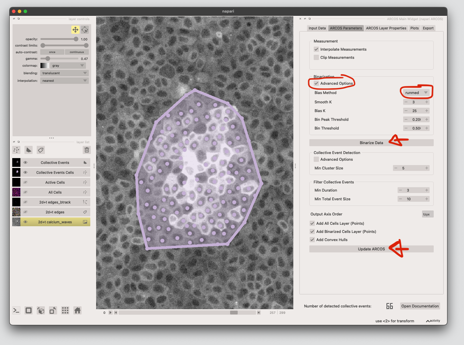
7. Detect collective events using ARCOS#
Load the tracking data and cell properties from the track and labels layer respectively. Click Load Data, and add the appropriate columns. We need the centroids for matching the labels and track layers, as well as the measurement column (mean is the mean calcium signal extracted in step 5.) X/Y columns might be switched, depending on which plugin you use to extract the features. Click Ok.

Next we run the ARCOS algorithm. Tick Advanced Options, select runmed as Bias Method, then click Binarize Data.
Finally click Update ARCOS to run!
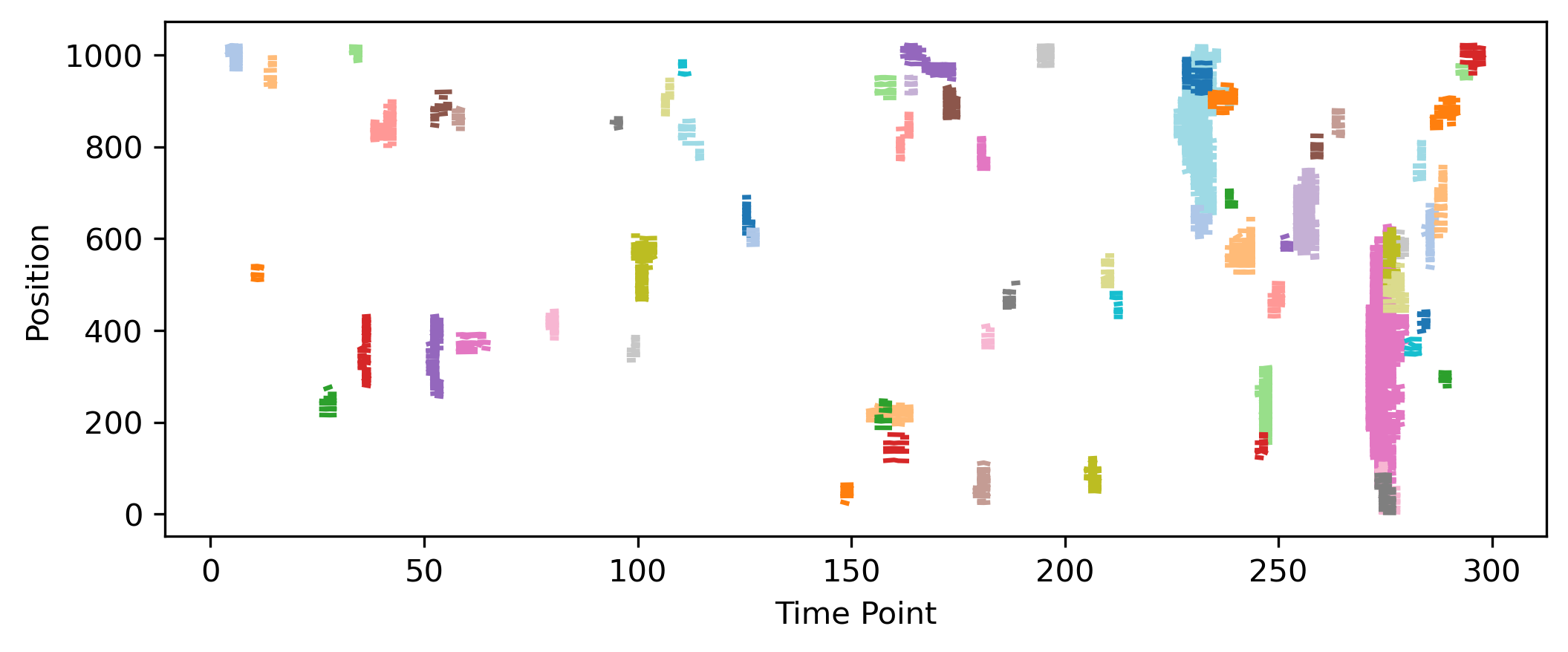
Plot ARCOS results#
First we import the results of ARCOS into this notebook.
from arcos_gui import get_current_arcos_plugin, get_arcos_output
from arcos4py.plotting import NoodlePlot
import pandas as pd
import matplotlib.pyplot as plt

# get the data from the napari ARCOS plugin
arcos_widget = get_current_arcos_plugin()
arcos_output, arcos_stats = get_arcos_output(arcos_widget)

# store the results as CSV
# arcos_output.to_csv('../sample_data/calcium_waves_workflow/arcos_output.csv', index=False)

# or load the output from file
# arcos_output = pd.read_csv('../sample_data/calcium_waves_workflow/arcos_output.csv')

arcos_output
fig = NoodlePlot(arcos_output, 'collid', 'track_id_factorized', 'frame', 'centroid_0', 'centroid_1').plot('centroid_0')

#change figure size
plt.gcf().set_size_inches(8,3)
plt.gcf().set_dpi(300)
If you want to export a movie, you can use the napari-timestamper plugin. This works from the GUI or with the following code:
import napari_timestamper

stack = napari_timestamper.render_as_rgb(viewer, axis=0)
napari_timestamper.save_image_stack(stack, directory= "../images/calcium_waves_workflow/",name="arcos_output", output_type="mp4")
Additional tips: Workflow as code instead of using the GUI#
Alternatively, the whole workflow can be run as code. To convert napari-assistant workflows to code snippets, click Generate code ..., then copy-paste to the jupyter notebook. To use the Convpaint API, refer to the tutorial in this documentation.
from tqdm import tqdm as tqdm
import pyclesperanto_prototype as cle

segmented = viewer.layers['segmented'].data
nb_frames = segmented.shape[0]

edges = []
for frame in tqdm(range(nb_frames)):
    # convert the Convpaint semantic segmentation to instance segmentation
    image1_vol = cle.voronoi_otsu_labeling(segmented[frame], None, 2.0, 2.0)

    # expand the labels by 2 pixels
    image1_E = cle.dilate_labels(image1_vol, None, 2.0)

    # reduce the labels to label edges
    image2_rltle = cle.reduce_labels_to_label_edges(image1_E)

    # expand the label edges by 2 pixels
    image3_elwmr = cle.dilate_labels(image2_rltle, None, 2.0)
    edges.append(image3_elwmr)

edges = np.array(edges)
viewer.add_labels(edges)