from napari_convpaint.conv_paint_model import ConvpaintModel
import numpy as np
import matplotlib.pyplot as plt
import skimage

Using Convpaint programmatically (API)

Loading a saved model and using it in a loop

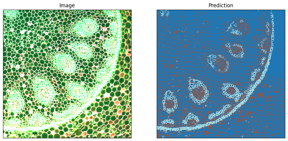
In one example workflow you might have interactively trained the model in the Napari GUI, and now want to use it programmatically in batch processing. Here we load a model trained on sample data and apply it to an image:

cpm = ConvpaintModel(model_path="../sample_data/lily_VGG16.pkl")

img = skimage.data.lily() # Load example image
img = np.moveaxis(img, -1, 0) # Move channel axis to first position, this is the convention throughout Convpaint

segmentation = cpm.segment(img)

For a simple illustration we extract the first 3 of the 4 channels of the image and display them as RGB. On the right, we show the predicted classes.

# Show the image and the annotations next to each other
fig, axes = plt.subplots(1, 2, figsize=(12, 6))

# Plot the image
axes[0].imshow(skimage.data.lily()[:,:,:3], cmap='gray')
axes[0].set_title('Image')

cmap = plt.get_cmap('tab20', 3)
cmap.set_under('white')

# Plot the prediction
axes[1].imshow(segmentation, cmap=cmap,interpolation='nearest')#,vmin=1,vmax=3)
axes[1].set_title('Prediction')

# Disable x and y ticks
for ax in axes:
    ax.set_xticks([])
    ax.set_yticks([])

Clipping input data to the valid range for imshow with RGB data ([0..1] for floats or [0..255] for integers). Got range [0..4095].

Creating and training a new model using the API

We can also create new models from scratch programatically. Like this, we can easily compare the performance of different models.

First let’s look at all the available feature extractors:

ConvpaintModel.get_fe_models_types()

{'vgg16': napari_convpaint.conv_paint_nnlayers.Hookmodel,
 'efficient_netb0': napari_convpaint.conv_paint_nnlayers.Hookmodel,
 'convnext': napari_convpaint.conv_paint_nnlayers.Hookmodel,
 'gaussian_features': napari_convpaint.conv_paint_gaussian.GaussianFeatures,
 'dinov2_vits14_reg': napari_convpaint.conv_paint_dino.DinoFeatures,
 'combo_dino_vgg': napari_convpaint.conv_paint_combo_fe.ComboFeatures,
 'combo_dino_gauss': napari_convpaint.conv_paint_combo_fe.ComboFeatures,
 'combo_dino_ilastik': napari_convpaint.conv_paint_combo_fe.ComboFeatures,
 'vit_small_patch14_reg4_dinov2': napari_convpaint.conv_paint_dino_jafar.DinoJafarFeatures,
 'cellpose_backbone': napari_convpaint.conv_paint_cellpose.CellposeFeatures,
 'ilastik_2d': napari_convpaint.conv_paint_ilastik.IlastikFeatures}

Tip: It's easy to implement your own feature extractor! Have a look at the file conv_paint_gaussian.py to see a minimal example. We've also provided a template file conv_paint_fe_template.py with instructions - you can copy and modify it to create your own feature extractor.

When using a CNN such as VGG16 as feature extractor, we need to supply the layers we want to use.

We can print out the selectable layers like this:

cpm2 = ConvpaintModel()
cpm2.get_fe_layer_keys()

['features.0 Conv2d(3, 64, kernel_size=(3, 3), stride=(1, 1), padding=(1, 1))',
 'features.2 Conv2d(64, 64, kernel_size=(3, 3), stride=(1, 1), padding=(1, 1))',
 'features.5 Conv2d(64, 128, kernel_size=(3, 3), stride=(1, 1), padding=(1, 1))',
 'features.7 Conv2d(128, 128, kernel_size=(3, 3), stride=(1, 1), padding=(1, 1))',
 'features.10 Conv2d(128, 256, kernel_size=(3, 3), stride=(1, 1), padding=(1, 1))',
 'features.12 Conv2d(256, 256, kernel_size=(3, 3), stride=(1, 1), padding=(1, 1))',
 'features.14 Conv2d(256, 256, kernel_size=(3, 3), stride=(1, 1), padding=(1, 1))',
 'features.17 Conv2d(256, 512, kernel_size=(3, 3), stride=(1, 1), padding=(1, 1))',
 'features.19 Conv2d(512, 512, kernel_size=(3, 3), stride=(1, 1), padding=(1, 1))',
 'features.21 Conv2d(512, 512, kernel_size=(3, 3), stride=(1, 1), padding=(1, 1))',
 'features.24 Conv2d(512, 512, kernel_size=(3, 3), stride=(1, 1), padding=(1, 1))',
 'features.26 Conv2d(512, 512, kernel_size=(3, 3), stride=(1, 1), padding=(1, 1))',
 'features.28 Conv2d(512, 512, kernel_size=(3, 3), stride=(1, 1), padding=(1, 1))']

By default, we’ve created a model using VGG16 with just the first layer for feature extraction:

cpm2.get_param("fe_layers")

['features.0 Conv2d(3, 64, kernel_size=(3, 3), stride=(1, 1), padding=(1, 1))']

Hint: The layers from VGG16 are filtered to only show layers of type Conv2D. Convpaint adds hooks at the selected layers, i.e. we capture their output. The flow through the network is interrupted at the last selected layer to speed up processing. Each hooked layer returns a certain number of outputs, which are then all concatenated into a single set of features.

Lets create a new VGG16 model using the first 2 layers. We store all the necessary settings in the ConvpaintModel object, which is also created in the background when using the napari plugin (GUI). Note that the layers can either be specified by names or as indices (among the available layers).

cpm3 = ConvpaintModel(fe_name="vgg16", fe_layers=[0, 1])
cpm3.get_param("fe_layers")

[0, 1]

Besides the layers for CNNs, there are several other options that can be set in the ConvpaintModel object:

• fe_scalings specifies the levels of downscaling to use for feature extraction (1 is the original size)

• fe_order specifies the spline order used to upscale small feature maps (either from the downscaling, or from aggregation in the neural network).

• with fe_use_min_features=True, only the n-first features of each output layer are selected, n being the number of features of the layer which outputs the least of them. This can help balance the weight of different layers.

• normalize will normalize the image so that it matches more closely the input expected by the pre-trained network.

• image_downsample allows to use a smaller version of the image as input. Note that this doesn’t change the size of the predicted output, as it gets rescaled to the original size in the end.

For a comprehensive description of all parameters and options, please refer to the separate page.

Let’s create a custom model. As you see below, except for the fe_name and layers (and gpu), all parameters can easily be adjusted after initialization - either one at a time, or multiples in one call:

cpm4 = ConvpaintModel(fe_name="vgg16", fe_layers=[0, 1])
cpm4.set_param("fe_scalings", [1, 2])

Train and test the model on artificial data:

# Create a noisy image
img = np.random.rand(200,200)
factor = 0.5
img[:50,:] = img[:50,:]*factor
img[80:100,:] = img[80:100,:]*factor

# Draw small rectangle as annotations 
annotations = np.zeros((200,200))
annotations[10:30,10:30] = 1      #class 1
annotations[170:190,170:190] = 2  #class 2

# Train the classifier to predict the annotations from the features
cpm4.train(img, annotations)

# Predict the annotations from the image
segmentation = cpm4.segment(img)

0:	learn: 0.5808966	total: 16.8ms	remaining: 1.67s
1:	learn: 0.4642788	total: 25.3ms	remaining: 1.24s
2:	learn: 0.3613301	total: 33.2ms	remaining: 1.07s
3:	learn: 0.2850847	total: 43.5ms	remaining: 1.04s
4:	learn: 0.2367290	total: 50ms	remaining: 951ms
5:	learn: 0.1967113	total: 57.4ms	remaining: 899ms
6:	learn: 0.1642987	total: 65.7ms	remaining: 873ms
7:	learn: 0.1331245	total: 72.1ms	remaining: 829ms
8:	learn: 0.1147539	total: 79.8ms	remaining: 806ms
9:	learn: 0.1012080	total: 86.2ms	remaining: 776ms
10:	learn: 0.0932405	total: 92.5ms	remaining: 749ms
11:	learn: 0.0832472	total: 99.6ms	remaining: 731ms
12:	learn: 0.0712612	total: 106ms	remaining: 710ms
13:	learn: 0.0634873	total: 113ms	remaining: 693ms
14:	learn: 0.0570575	total: 119ms	remaining: 677ms
15:	learn: 0.0535091	total: 126ms	remaining: 663ms
16:	learn: 0.0489758	total: 133ms	remaining: 648ms
17:	learn: 0.0433077	total: 139ms	remaining: 633ms
18:	learn: 0.0397668	total: 145ms	remaining: 618ms
19:	learn: 0.0365790	total: 151ms	remaining: 605ms
20:	learn: 0.0334537	total: 158ms	remaining: 595ms
21:	learn: 0.0300977	total: 165ms	remaining: 586ms
22:	learn: 0.0278731	total: 172ms	remaining: 576ms
23:	learn: 0.0246787	total: 178ms	remaining: 564ms
24:	learn: 0.0222810	total: 184ms	remaining: 553ms
25:	learn: 0.0212631	total: 191ms	remaining: 543ms
26:	learn: 0.0187676	total: 197ms	remaining: 533ms
27:	learn: 0.0175589	total: 203ms	remaining: 522ms
28:	learn: 0.0158279	total: 210ms	remaining: 514ms
29:	learn: 0.0145287	total: 216ms	remaining: 504ms
30:	learn: 0.0132551	total: 222ms	remaining: 495ms
31:	learn: 0.0126037	total: 228ms	remaining: 486ms
32:	learn: 0.0118544	total: 235ms	remaining: 476ms
33:	learn: 0.0112698	total: 241ms	remaining: 468ms
34:	learn: 0.0104152	total: 248ms	remaining: 461ms
35:	learn: 0.0099372	total: 255ms	remaining: 453ms
36:	learn: 0.0094620	total: 263ms	remaining: 447ms
37:	learn: 0.0088299	total: 269ms	remaining: 438ms
38:	learn: 0.0082279	total: 277ms	remaining: 433ms
39:	learn: 0.0078590	total: 283ms	remaining: 425ms
40:	learn: 0.0075439	total: 290ms	remaining: 417ms
41:	learn: 0.0072947	total: 296ms	remaining: 409ms
42:	learn: 0.0067791	total: 302ms	remaining: 400ms
43:	learn: 0.0063790	total: 309ms	remaining: 393ms
44:	learn: 0.0058580	total: 315ms	remaining: 386ms
45:	learn: 0.0055641	total: 322ms	remaining: 378ms
46:	learn: 0.0052643	total: 328ms	remaining: 370ms
47:	learn: 0.0050223	total: 334ms	remaining: 362ms
48:	learn: 0.0047752	total: 341ms	remaining: 355ms
49:	learn: 0.0045167	total: 347ms	remaining: 347ms
50:	learn: 0.0042964	total: 353ms	remaining: 340ms
51:	learn: 0.0041689	total: 360ms	remaining: 332ms
52:	learn: 0.0040102	total: 366ms	remaining: 324ms
53:	learn: 0.0038869	total: 372ms	remaining: 317ms
54:	learn: 0.0037075	total: 378ms	remaining: 309ms
55:	learn: 0.0035237	total: 384ms	remaining: 302ms
56:	learn: 0.0033846	total: 391ms	remaining: 295ms
57:	learn: 0.0032610	total: 397ms	remaining: 287ms
58:	learn: 0.0030956	total: 403ms	remaining: 280ms
59:	learn: 0.0029692	total: 409ms	remaining: 273ms
60:	learn: 0.0028744	total: 415ms	remaining: 265ms
61:	learn: 0.0027833	total: 421ms	remaining: 258ms
62:	learn: 0.0027079	total: 427ms	remaining: 251ms
63:	learn: 0.0026149	total: 434ms	remaining: 244ms
64:	learn: 0.0025087	total: 441ms	remaining: 237ms
65:	learn: 0.0024284	total: 446ms	remaining: 230ms
66:	learn: 0.0023439	total: 453ms	remaining: 223ms
67:	learn: 0.0022735	total: 459ms	remaining: 216ms
68:	learn: 0.0021950	total: 465ms	remaining: 209ms
69:	learn: 0.0021204	total: 472ms	remaining: 202ms
70:	learn: 0.0020509	total: 479ms	remaining: 195ms
71:	learn: 0.0019904	total: 485ms	remaining: 189ms
72:	learn: 0.0019349	total: 491ms	remaining: 182ms
73:	learn: 0.0018856	total: 498ms	remaining: 175ms
74:	learn: 0.0018403	total: 504ms	remaining: 168ms
75:	learn: 0.0017821	total: 510ms	remaining: 161ms
76:	learn: 0.0017449	total: 517ms	remaining: 154ms
77:	learn: 0.0017026	total: 523ms	remaining: 147ms
78:	learn: 0.0016640	total: 529ms	remaining: 141ms
79:	learn: 0.0016168	total: 535ms	remaining: 134ms
80:	learn: 0.0015818	total: 541ms	remaining: 127ms
81:	learn: 0.0015479	total: 547ms	remaining: 120ms
82:	learn: 0.0015054	total: 554ms	remaining: 113ms
83:	learn: 0.0014698	total: 560ms	remaining: 107ms
84:	learn: 0.0014295	total: 566ms	remaining: 99.9ms
85:	learn: 0.0013924	total: 573ms	remaining: 93.2ms
86:	learn: 0.0013567	total: 579ms	remaining: 86.5ms
87:	learn: 0.0013234	total: 585ms	remaining: 79.8ms
88:	learn: 0.0012930	total: 591ms	remaining: 73ms
89:	learn: 0.0012649	total: 597ms	remaining: 66.3ms
90:	learn: 0.0012365	total: 603ms	remaining: 59.7ms
91:	learn: 0.0012364	total: 609ms	remaining: 53ms
92:	learn: 0.0012099	total: 615ms	remaining: 46.3ms
93:	learn: 0.0011846	total: 621ms	remaining: 39.7ms
94:	learn: 0.0011536	total: 628ms	remaining: 33ms
95:	learn: 0.0011533	total: 634ms	remaining: 26.4ms
96:	learn: 0.0011313	total: 640ms	remaining: 19.8ms
97:	learn: 0.0011113	total: 646ms	remaining: 13.2ms
98:	learn: 0.0011113	total: 652ms	remaining: 6.59ms
99:	learn: 0.0011112	total: 658ms	remaining: 0us

# Show the image and the annotations
fig, axes = plt.subplots(1, 3, figsize=(12, 6))

# Plot the image
axes[0].imshow(img, cmap='gray')
axes[0].set_title('Image')

cmap = plt.get_cmap('tab20')
cmap.set_under('white')
# Plot the annotations
axes[1].imshow(annotations, cmap=cmap,interpolation='nearest',vmin=1,vmax=3)
axes[1].set_title('Annotations')

# Plot the prediction
axes[2].imshow(segmentation, cmap=cmap,interpolation='nearest',vmin=1,vmax=3)
axes[2].set_title('Prediction')

# Disable x and y ticks
for ax in axes:
    ax.set_xticks([])
    ax.set_yticks([])

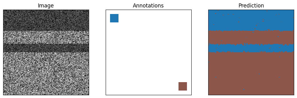
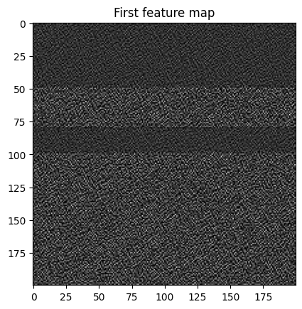
The selected output layers have 64 and 64 output features and we’re using three scalings, so in total we have (64+64)*3 = 384 features. With our ConvpaintModel, we can also extract those features to display and analyze them further:

features = cpm4.get_feature_image(img)
print(f"Number of features: {features.shape}")
plt.imshow(features[0], cmap='gray')
plt.title('First feature map')
plt.show()

Number of features: (256, 200, 200)

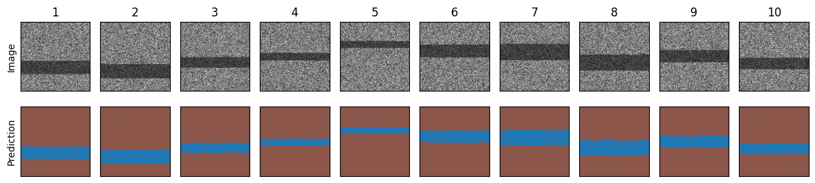
Running Convpaint in a loop for batch processing

num_images = 10 # Number of images to generate

imgs = []
segmentations = []

for i in range(num_images):
    # Create a noisy image
    img = np.random.rand(200, 200)
    start_row = np.random.randint(0, 150)
    end_row = start_row + np.random.randint(20, 50)
    img[start_row:end_row, :] = img[start_row:end_row, :] * 0.5
    
    # Make prediction
    segmentation = cpm4.segment(img)
    
    imgs.append(img)
    segmentations.append(segmentation)

# Create a figure with a grid of subplots
fig, axs = plt.subplots(2, num_images, figsize=(12, 3))

for i in range(num_images):
    # Plot sample image
    axs[0, i].imshow(imgs[i], cmap='gray')
    axs[0, i].set_title(f'{i+1}')
    axs[0, i].set_xticks([])
    axs[0, i].set_yticks([])


    
    # Plot prediction
    axs[1, i].imshow(segmentations[i], cmap=cmap, interpolation='nearest', vmin=1, vmax=3)
    axs[1, i].set_title(f'')
    axs[1, i].set_xticks([])
    axs[1, i].set_yticks([])


# Add y labels
axs[0, 0].set_ylabel('Image')
axs[1, 0].set_ylabel('Prediction')

plt.tight_layout()
plt.show()

Note: In Pertz Lab we train a model using the GUI on data live streamed from the microscope at the beginning of an experiment. The trained model is then used programmatically for smart microscopy approaches, for example enabling optogenetic stimulation of subcellular areas, or automated selection of cells that fit a certain shape criteria.

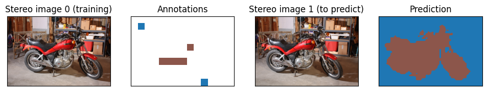
Creating a model using DINOv2 as feature extractor

For the ViT based DINOv2 model we’re not selecting the layers, and instead just extract all patch based features.

Note that this time, we are using another option to initialize a ConvpaintModel (just for illustration purposes; you could also use the initialization method described above). Using an alias to create a pre-defined model is in fact the simplest way to get started with Convpaint. For details, refer to the Feature Extractor page.

Importantly, here we are handling images with an additional dimension. Hence, we need to tell the model what that dimension represents: a third “spatial” dimension (in particular z or time), or a “channel” dimension (for example, RGB color channels). Here, we set multi_channel_img to True in accordance with the RGB color channels of the image.

cpm_dino = ConvpaintModel(alias="dino")
cpm_dino.set_param("multi_channel_img", True)

# Create new dataset
img = skimage.data.stereo_motorcycle()
train_img = np.moveaxis(img[0], -1, 0)
pred_img = np.moveaxis(img[1], -1, 0)
annotations = np.zeros(img[0][:,:,0].shape)
# Foreground [y,x]
annotations[50:100,50:100] = 1
annotations[450:500,500:550] = 1
# Background [x,y]
annotations[200:250,400:450] = 2
annotations[300:350,200:400] = 2

# Train the model
cpm_dino.train(train_img, annotations)

# Use it to segment the image
segmentation = cpm_dino.segment(image=pred_img)

C:\Users\roman\Documents\Convpaint\hinderling-cp\napari-convpaint\src\napari_convpaint\conv_paint_model.py:1522: UserWarning: Annotations for image 0 are not of type int. Converting to int32.
  warnings.warn(f'Annotations for image {i} are not of type int. Converting to int32.')

0:	learn: 0.3768599	total: 34.2ms	remaining: 3.38s
1:	learn: 0.2002017	total: 50.3ms	remaining: 2.47s
2:	learn: 0.1085167	total: 66.7ms	remaining: 2.15s
3:	learn: 0.0631080	total: 81.4ms	remaining: 1.95s
4:	learn: 0.0358521	total: 95.5ms	remaining: 1.81s
5:	learn: 0.0219060	total: 110ms	remaining: 1.73s
6:	learn: 0.0140858	total: 142ms	remaining: 1.89s
7:	learn: 0.0092302	total: 159ms	remaining: 1.82s
8:	learn: 0.0062938	total: 173ms	remaining: 1.75s
9:	learn: 0.0045885	total: 187ms	remaining: 1.68s
10:	learn: 0.0032304	total: 199ms	remaining: 1.61s
11:	learn: 0.0024106	total: 212ms	remaining: 1.55s
12:	learn: 0.0018580	total: 224ms	remaining: 1.5s
13:	learn: 0.0014287	total: 237ms	remaining: 1.45s
14:	learn: 0.0011273	total: 249ms	remaining: 1.41s
15:	learn: 0.0009283	total: 262ms	remaining: 1.37s
16:	learn: 0.0007666	total: 275ms	remaining: 1.34s
17:	learn: 0.0006563	total: 287ms	remaining: 1.31s
18:	learn: 0.0005687	total: 299ms	remaining: 1.27s
19:	learn: 0.0004960	total: 324ms	remaining: 1.29s
20:	learn: 0.0004467	total: 335ms	remaining: 1.26s
21:	learn: 0.0004095	total: 347ms	remaining: 1.23s
22:	learn: 0.0003607	total: 358ms	remaining: 1.2s
23:	learn: 0.0003323	total: 370ms	remaining: 1.17s
24:	learn: 0.0003091	total: 382ms	remaining: 1.15s
25:	learn: 0.0002905	total: 393ms	remaining: 1.12s
26:	learn: 0.0002741	total: 404ms	remaining: 1.09s
27:	learn: 0.0002594	total: 416ms	remaining: 1.07s
28:	learn: 0.0002490	total: 427ms	remaining: 1.04s
29:	learn: 0.0002490	total: 439ms	remaining: 1.02s
30:	learn: 0.0002490	total: 450ms	remaining: 1s
31:	learn: 0.0002490	total: 462ms	remaining: 981ms
32:	learn: 0.0002227	total: 474ms	remaining: 962ms
33:	learn: 0.0002151	total: 485ms	remaining: 942ms
34:	learn: 0.0001998	total: 497ms	remaining: 923ms
35:	learn: 0.0001998	total: 508ms	remaining: 903ms
36:	learn: 0.0001998	total: 519ms	remaining: 884ms
37:	learn: 0.0001998	total: 530ms	remaining: 864ms
38:	learn: 0.0001997	total: 540ms	remaining: 845ms
39:	learn: 0.0001998	total: 551ms	remaining: 827ms
40:	learn: 0.0001998	total: 563ms	remaining: 810ms
41:	learn: 0.0001969	total: 575ms	remaining: 794ms
42:	learn: 0.0001933	total: 587ms	remaining: 779ms
43:	learn: 0.0001933	total: 599ms	remaining: 762ms
44:	learn: 0.0001932	total: 610ms	remaining: 746ms
45:	learn: 0.0001895	total: 622ms	remaining: 730ms
46:	learn: 0.0001894	total: 633ms	remaining: 714ms
47:	learn: 0.0001862	total: 644ms	remaining: 698ms
48:	learn: 0.0001861	total: 656ms	remaining: 682ms
49:	learn: 0.0001861	total: 667ms	remaining: 667ms
50:	learn: 0.0001861	total: 678ms	remaining: 652ms
51:	learn: 0.0001860	total: 689ms	remaining: 636ms
52:	learn: 0.0001860	total: 700ms	remaining: 621ms
53:	learn: 0.0001860	total: 711ms	remaining: 606ms
54:	learn: 0.0001860	total: 722ms	remaining: 591ms
55:	learn: 0.0001860	total: 733ms	remaining: 576ms
56:	learn: 0.0001859	total: 744ms	remaining: 561ms
57:	learn: 0.0001859	total: 755ms	remaining: 546ms
58:	learn: 0.0001860	total: 766ms	remaining: 532ms
59:	learn: 0.0001859	total: 777ms	remaining: 518ms
60:	learn: 0.0001859	total: 788ms	remaining: 504ms
61:	learn: 0.0001825	total: 799ms	remaining: 490ms
62:	learn: 0.0001791	total: 810ms	remaining: 476ms
63:	learn: 0.0001791	total: 820ms	remaining: 461ms
64:	learn: 0.0001763	total: 831ms	remaining: 448ms
65:	learn: 0.0001763	total: 843ms	remaining: 434ms
66:	learn: 0.0001730	total: 854ms	remaining: 421ms
67:	learn: 0.0001730	total: 865ms	remaining: 407ms
68:	learn: 0.0001730	total: 876ms	remaining: 394ms
69:	learn: 0.0001730	total: 888ms	remaining: 381ms
70:	learn: 0.0001729	total: 899ms	remaining: 367ms
71:	learn: 0.0001729	total: 913ms	remaining: 355ms
72:	learn: 0.0001679	total: 924ms	remaining: 342ms
73:	learn: 0.0001679	total: 935ms	remaining: 329ms
74:	learn: 0.0001680	total: 947ms	remaining: 316ms
75:	learn: 0.0001680	total: 958ms	remaining: 303ms
76:	learn: 0.0001680	total: 969ms	remaining: 290ms
77:	learn: 0.0001680	total: 981ms	remaining: 277ms
78:	learn: 0.0001680	total: 992ms	remaining: 264ms
79:	learn: 0.0001680	total: 1s	remaining: 251ms
80:	learn: 0.0001679	total: 1.01s	remaining: 238ms
81:	learn: 0.0001680	total: 1.03s	remaining: 225ms
82:	learn: 0.0001620	total: 1.04s	remaining: 212ms
83:	learn: 0.0001620	total: 1.05s	remaining: 200ms
84:	learn: 0.0001620	total: 1.06s	remaining: 187ms
85:	learn: 0.0001620	total: 1.07s	remaining: 174ms
86:	learn: 0.0001619	total: 1.08s	remaining: 161ms
87:	learn: 0.0001619	total: 1.09s	remaining: 149ms
88:	learn: 0.0001619	total: 1.1s	remaining: 136ms
89:	learn: 0.0001619	total: 1.13s	remaining: 125ms
90:	learn: 0.0001620	total: 1.14s	remaining: 113ms
91:	learn: 0.0001619	total: 1.15s	remaining: 100ms
92:	learn: 0.0001620	total: 1.16s	remaining: 87.4ms
93:	learn: 0.0001620	total: 1.17s	remaining: 74.8ms
94:	learn: 0.0001619	total: 1.18s	remaining: 62.3ms
95:	learn: 0.0001620	total: 1.19s	remaining: 49.8ms
96:	learn: 0.0001620	total: 1.21s	remaining: 37.3ms
97:	learn: 0.0001619	total: 1.22s	remaining: 24.8ms
98:	learn: 0.0001619	total: 1.23s	remaining: 12.4ms
99:	learn: 0.0001619	total: 1.24s	remaining: 0us

# Show the image and the annotations
fig, axes = plt.subplots(1, 4, figsize=(12, 8))

# Plot the image
axes[0].imshow(img[0], cmap='gray')
axes[0].set_title(f'Stereo image 0 (training)')

cmap = plt.get_cmap('tab20')
cmap.set_under('white')

# Plot the annotations
axes[1].imshow(annotations, cmap=cmap, interpolation='nearest', vmin=1, vmax=3)
axes[1].set_title('Annotations')

# Plot the image to predict
axes[2].imshow(img[1], cmap='gray')
axes[2].set_title(f'Stereo image 1 (to predict)')


# Plot the prediction
axes[3].imshow(segmentation, cmap=cmap, interpolation='nearest', vmin=1, vmax=3)
axes[3].set_title('Prediction')

# Disable x and y ticks
for ax in axes:
    ax.set_xticks([])
    ax.set_yticks([])

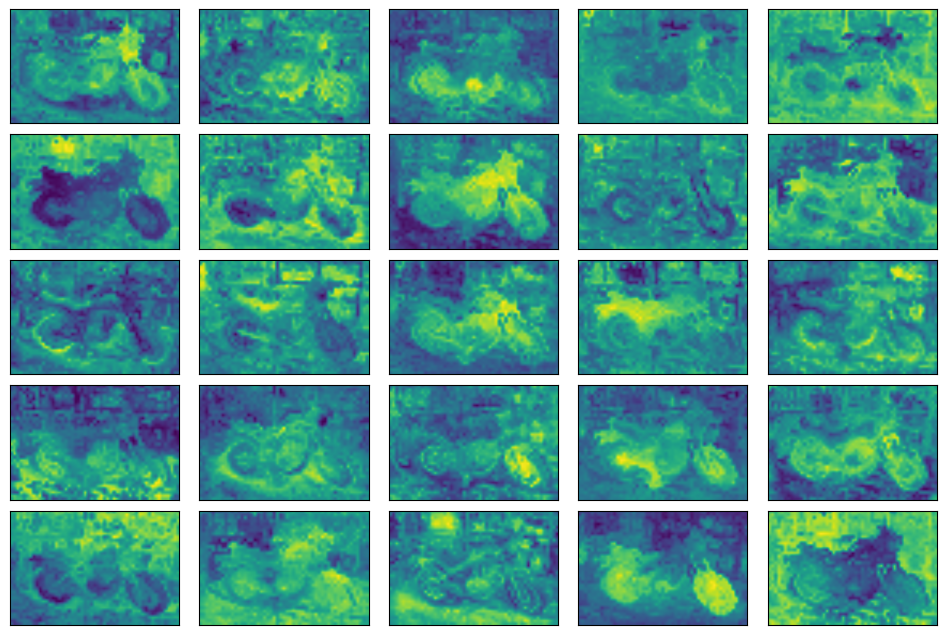
Visualizing the extracted DINOv2 features

feature_image = cpm_dino.get_feature_image(train_img)

num_features = feature_image.shape[0]
print(f"Extracted {num_features} features.")

grid_size = 5
random_features = np.random.choice(num_features, grid_size*grid_size)
fig, axes = plt.subplots(grid_size, grid_size, figsize=(12, 8))
for i, ax in enumerate(axes.flat):
    ax.imshow(feature_image[random_features[i]], cmap='viridis')
    ax.set_xticks([])
    ax.set_yticks([])
    
# Set w/h distance between subplots to 0
plt.subplots_adjust(wspace=0.1, hspace=0.1)

Extracted 384 features.

Tip: It can be useful to visualize the extracted features for troubleshooting and getting an intuition for the level of detail that the model considers. In this example, DINOv2 extracts high-level semantic features like tires, floor, bike body or engine.

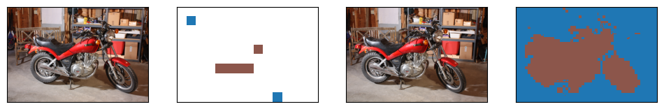
Combining features from multiple models

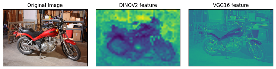
The strengths of different feature extractors can be combined by concatenating their outputs. For example, the good spatial resolution of VGG16 can be combined with the rich semantic features of DINOv2. This leads to very successful segmentations on some datasets.

We are providing a selection of pre-defined combo feature extractors. You can use these out of the box or as a starting point for your own custom configurations.

cpm_combo = ConvpaintModel(fe_name="combo_dino_vgg", multi_channel_img=True)

train_img = np.moveaxis(skimage.data.stereo_motorcycle()[0],-1,0)
pred_img = np.moveaxis(skimage.data.stereo_motorcycle()[1],-1,0) 

# Train on the first image
cpm_combo.train(train_img, annotations)

# Predict on the second
segmentation = cpm_combo.segment(pred_img)

C:\Users\roman\Documents\Convpaint\hinderling-cp\napari-convpaint\src\napari_convpaint\conv_paint_model.py:1522: UserWarning: Annotations for image 0 are not of type int. Converting to int32.
  warnings.warn(f'Annotations for image {i} are not of type int. Converting to int32.')

0:	learn: 0.3776222	total: 27.2ms	remaining: 2.69s
1:	learn: 0.2040664	total: 48.8ms	remaining: 2.39s
2:	learn: 0.1180317	total: 68.9ms	remaining: 2.23s
3:	learn: 0.0671248	total: 87.3ms	remaining: 2.1s
4:	learn: 0.0386676	total: 106ms	remaining: 2.01s
5:	learn: 0.0246967	total: 123ms	remaining: 1.93s
6:	learn: 0.0151749	total: 141ms	remaining: 1.87s
7:	learn: 0.0097853	total: 157ms	remaining: 1.81s
8:	learn: 0.0067584	total: 174ms	remaining: 1.76s
9:	learn: 0.0044729	total: 191ms	remaining: 1.72s
10:	learn: 0.0031835	total: 208ms	remaining: 1.68s
11:	learn: 0.0022336	total: 224ms	remaining: 1.64s
12:	learn: 0.0017226	total: 242ms	remaining: 1.62s
13:	learn: 0.0013815	total: 260ms	remaining: 1.6s
14:	learn: 0.0011009	total: 278ms	remaining: 1.57s
15:	learn: 0.0008923	total: 296ms	remaining: 1.56s
16:	learn: 0.0007368	total: 313ms	remaining: 1.53s
17:	learn: 0.0006244	total: 330ms	remaining: 1.5s
18:	learn: 0.0005451	total: 345ms	remaining: 1.47s
19:	learn: 0.0004590	total: 362ms	remaining: 1.45s
20:	learn: 0.0003852	total: 374ms	remaining: 1.41s
21:	learn: 0.0003405	total: 391ms	remaining: 1.39s
22:	learn: 0.0003008	total: 408ms	remaining: 1.37s
23:	learn: 0.0002705	total: 426ms	remaining: 1.35s
24:	learn: 0.0002351	total: 443ms	remaining: 1.33s
25:	learn: 0.0002105	total: 460ms	remaining: 1.31s
26:	learn: 0.0002021	total: 477ms	remaining: 1.29s
27:	learn: 0.0002021	total: 493ms	remaining: 1.27s
28:	learn: 0.0001906	total: 510ms	remaining: 1.25s
29:	learn: 0.0001906	total: 526ms	remaining: 1.23s
30:	learn: 0.0001905	total: 542ms	remaining: 1.21s
31:	learn: 0.0001905	total: 559ms	remaining: 1.19s
32:	learn: 0.0001905	total: 576ms	remaining: 1.17s
33:	learn: 0.0001905	total: 593ms	remaining: 1.15s
34:	learn: 0.0001905	total: 609ms	remaining: 1.13s
35:	learn: 0.0001905	total: 625ms	remaining: 1.11s
36:	learn: 0.0001905	total: 637ms	remaining: 1.08s
37:	learn: 0.0001905	total: 653ms	remaining: 1.06s
38:	learn: 0.0001702	total: 666ms	remaining: 1.04s
39:	learn: 0.0001702	total: 682ms	remaining: 1.02s
40:	learn: 0.0001702	total: 699ms	remaining: 1s
41:	learn: 0.0001702	total: 715ms	remaining: 987ms
42:	learn: 0.0001702	total: 731ms	remaining: 969ms
43:	learn: 0.0001639	total: 747ms	remaining: 951ms
44:	learn: 0.0001639	total: 763ms	remaining: 933ms
45:	learn: 0.0001639	total: 779ms	remaining: 914ms
46:	learn: 0.0001639	total: 795ms	remaining: 897ms
47:	learn: 0.0001639	total: 811ms	remaining: 879ms
48:	learn: 0.0001639	total: 828ms	remaining: 862ms
49:	learn: 0.0001639	total: 843ms	remaining: 843ms
50:	learn: 0.0001639	total: 859ms	remaining: 826ms
51:	learn: 0.0001639	total: 874ms	remaining: 807ms
52:	learn: 0.0001639	total: 890ms	remaining: 789ms
53:	learn: 0.0001639	total: 906ms	remaining: 772ms
54:	learn: 0.0001639	total: 921ms	remaining: 754ms
55:	learn: 0.0001639	total: 938ms	remaining: 737ms
56:	learn: 0.0001638	total: 954ms	remaining: 720ms
57:	learn: 0.0001638	total: 970ms	remaining: 703ms
58:	learn: 0.0001638	total: 986ms	remaining: 685ms
59:	learn: 0.0001638	total: 1s	remaining: 668ms
60:	learn: 0.0001638	total: 1.02s	remaining: 650ms
61:	learn: 0.0001638	total: 1.03s	remaining: 633ms
62:	learn: 0.0001638	total: 1.05s	remaining: 616ms
63:	learn: 0.0001638	total: 1.06s	remaining: 599ms
64:	learn: 0.0001638	total: 1.08s	remaining: 582ms
65:	learn: 0.0001638	total: 1.1s	remaining: 566ms
66:	learn: 0.0001638	total: 1.11s	remaining: 549ms
67:	learn: 0.0001638	total: 1.13s	remaining: 532ms
68:	learn: 0.0001638	total: 1.15s	remaining: 515ms
69:	learn: 0.0001638	total: 1.16s	remaining: 498ms
70:	learn: 0.0001606	total: 1.18s	remaining: 480ms
71:	learn: 0.0001605	total: 1.19s	remaining: 463ms
72:	learn: 0.0001605	total: 1.21s	remaining: 447ms
73:	learn: 0.0001606	total: 1.22s	remaining: 430ms
74:	learn: 0.0001606	total: 1.24s	remaining: 413ms
75:	learn: 0.0001606	total: 1.25s	remaining: 396ms
76:	learn: 0.0001605	total: 1.27s	remaining: 379ms
77:	learn: 0.0001576	total: 1.28s	remaining: 363ms
78:	learn: 0.0001576	total: 1.3s	remaining: 346ms
79:	learn: 0.0001576	total: 1.32s	remaining: 329ms
80:	learn: 0.0001576	total: 1.33s	remaining: 312ms
81:	learn: 0.0001577	total: 1.35s	remaining: 296ms
82:	learn: 0.0001576	total: 1.36s	remaining: 279ms
83:	learn: 0.0001576	total: 1.38s	remaining: 263ms
84:	learn: 0.0001576	total: 1.39s	remaining: 246ms
85:	learn: 0.0001393	total: 1.41s	remaining: 230ms
86:	learn: 0.0001393	total: 1.43s	remaining: 213ms
87:	learn: 0.0001393	total: 1.44s	remaining: 197ms
88:	learn: 0.0001393	total: 1.46s	remaining: 180ms
89:	learn: 0.0001393	total: 1.47s	remaining: 164ms
90:	learn: 0.0001393	total: 1.49s	remaining: 147ms
91:	learn: 0.0001393	total: 1.5s	remaining: 131ms
92:	learn: 0.0001393	total: 1.52s	remaining: 114ms
93:	learn: 0.0001393	total: 1.54s	remaining: 98.1ms
94:	learn: 0.0001393	total: 1.55s	remaining: 81.7ms
95:	learn: 0.0001393	total: 1.57s	remaining: 65.3ms
96:	learn: 0.0001393	total: 1.58s	remaining: 49ms
97:	learn: 0.0001393	total: 1.6s	remaining: 32.6ms
98:	learn: 0.0001393	total: 1.61s	remaining: 16.3ms
99:	learn: 0.0001393	total: 1.63s	remaining: 0us

# Show the image and the annotations
fig, axes = plt.subplots(1, 4, figsize=(12, 6))

# Plot the image
axes[0].imshow(img[0], cmap='gray')

cmap = plt.get_cmap('tab20')
cmap.set_under('white')

# Plot the annotations
axes[1].imshow(annotations, cmap=cmap, interpolation='nearest', vmin=1, vmax=3)

# Plot the image to predict
axes[2].imshow(img[1], cmap='gray')

# Plot the prediction
axes[3].imshow(segmentation, cmap=cmap, interpolation='nearest', vmin=1, vmax=3)

# Disable x and y ticks
for ax in axes:
    ax.set_xticks([])
    ax.set_yticks([])

Visual comparison of features extracted by DINOv2 vs. VGG16

cpm_vgg = ConvpaintModel(fe_name="vgg16", multi_channel_img=True)
features_vgg = cpm_vgg.get_feature_image(train_img)

cpm_dino = ConvpaintModel(fe_name="dinov2_vits14_reg", multi_channel_img=True)
features_dino = cpm_dino.get_feature_image(train_img)

fig, axes = plt.subplots(1, 3, figsize=(12, 12))

# Plot img, and a random feature each from dinov2 and vgg16
axes[1].imshow(features_dino[22,:,:], cmap='viridis')
axes[1].set_title('DINOV2 feature')
axes[2].imshow(features_vgg[22,:,:], cmap='viridis')
axes[2].set_title('VGG16 feature')
axes[0].imshow(img[0])
axes[0].set_title('Original Image')
for ax in axes:
    ax.set_xticks([])
    ax.set_yticks([])

plt.subplots_adjust(wspace=0.1, hspace=0.1)