14. U-net
Contents
![]()
14. U-net
Until now we have only seen reasonably small and simple networks. Most real networks are much larger and complex and we are going to see how one implement such a network here, namely the U-net.
The U-net (U-Net: Convolutional Networks for Biomedical Image Segmentation, Ronneberger et al. 2015) is one of the most popular architecture used for segmentation. It is a fully convolutional network bringing the additional advantage that it is not limited to a certain image size. It takes its name from its visual representation where a encoder downsizing the input is followed by a decoder increasing it again:
from IPython.display import Image

# set path containing data folder or use default for Colab (/gdrive/My Drive)
local_folder = "../"
import urllib.request
urllib.request.urlretrieve('https://raw.githubusercontent.com/guiwitz/DLImaging/master/utils/check_colab.py', 'check_colab.py')
from check_colab import set_datapath
colab, datapath = set_datapath(local_folder)
Image(url='https://github.com/guiwitz/DLImaging/raw/master/illustrations/unet.jpg', width=800)

As can be seen in the graphics above, the U-net is composed of a series of convolutional layers followed by activations and max-pooling for the encoding part and a series of convolutional layers followed by activations up-convolutions (transpose convolutions). This is very similar to the sort of architecture we have seen in the Autoencoder notebook.
However, additionally, in the decoding part, layers from the encoder are directly concatenated with layers from the decoder. Encoder-decoder architecture often have the problem that small-scale details are lost (see previous chapter), and these skip-connections correct for that by adding back layers where these details have not been “washed-out” yet.
Implementation
For the sake of simplicity, we are creating here a very simple Unet, with just one convolution per depth and with only one depth level. Our input is a single image. We load one and apply the necessary transform:
from pathlib import Path

import torch
from torch import nn
from torch.functional import F
from torchvision import transforms
from torch.utils.data import Dataset, DataLoader, random_split
import pytorch_lightning as pl
from pytorch_lightning.loggers import TensorBoardLogger

from sklearn.metrics import jaccard_score

import skimage.io
import matplotlib.pyplot as plt
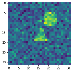
We load an image as an example:
image = skimage.io.imread(datapath.joinpath('data/triangle_circle_noisy_seg/images/image_0.tif'))
We define a transform for our image:
transform = transforms.Compose([transforms.ToTensor()])
im_tensor = transform(image)
im_batch = im_tensor.unsqueeze(0)
im_batch.shape
torch.Size([1, 1, 32, 32])
plt.imshow(image);
Now we create the first convolution layer of the first depth level. We also apply ReLU on the output:
conv1 = nn.Conv2d(in_channels=1, out_channels=16, kernel_size=3, padding=1)
x1 = F.relu(conv1(im_batch))
Note that unlike what we did previously, passing a x variables across layers, we will give specific names to the outputs of different layers. We need that so that we can use those layers in the skip-connections!
Now we have a max-pooling layer:
maxpool1 = nn.MaxPool2d(kernel_size=2)
x = maxpool1(x1)
x.shape
torch.Size([1, 16, 16, 16])
Now we can do two new rounds of convolution/pooling. We double the number of filters while we halve the image size:
conv2 = nn.Conv2d(in_channels=16, out_channels=32, kernel_size=3, padding=1)
maxpool2 = nn.MaxPool2d(kernel_size=2)
conv3 = nn.Conv2d(in_channels=32, out_channels=64, kernel_size=3, padding=1)
x2 = F.relu(conv2(x))
x = maxpool2(x2)
x3 = F.relu(conv3(x))
x3.shape
torch.Size([1, 64, 8, 8])
We have arrived at the “bottom” of the Unet. Now we have to do the reverse step. And don’t forget to add the skip connections! First, we do an up-convolution:
transpose_conv3 = nn.ConvTranspose2d(in_channels=64, out_channels=32, kernel_size=2, padding=0, stride=2)
x2_t = transpose_conv3(x3)
x2_t.shape
torch.Size([1, 32, 16, 16])
Now we can combine this with the x2 output which has the same size:
x2.shape
torch.Size([1, 32, 16, 16])
For that we concatenate the two outputs:
x = torch.cat((x2, x2_t),dim=1)
x.shape
torch.Size([1, 64, 16, 16])
Finally we add the convolution layer at that depth:
conv2_t = nn.Conv2d(in_channels=64, out_channels=32, kernel_size=3, padding=1)
x = F.relu(conv2_t(x))
x.shape
torch.Size([1, 32, 16, 16])
Now we repeat the operation:
transpose_conv2 = nn.ConvTranspose2d(in_channels=32, out_channels=16, kernel_size=2, padding=0, stride=2)
conv1_t = nn.Conv2d(in_channels=32, out_channels=16, kernel_size=3, padding=1)
x = transpose_conv2(x)
x = torch.cat((x1, x),dim=1)
x = F.relu(conv1_t(x))
x.shape
torch.Size([1, 16, 32, 32])
So we are back to our original size! The last thing we have to do is reduce our stack of size 16 to the number of classes used in the segmentation that we can then use for e.g. soft-max:
num_classes = 3

conv_final = nn.Conv2d(in_channels=16, out_channels=num_classes, kernel_size=1)
x = conv_final(x)
x.shape
torch.Size([1, 3, 32, 32])
Assembling in a module
We can now assemble all these steps in a Lightning module as we have done before:
class Unet(pl.LightningModule):
    def __init__(self, num_classes, learning_rate):
        super(Unet, self).__init__()

        self.conv1 = nn.Conv2d(in_channels=1, out_channels=16, kernel_size=3, padding=1)
        self.maxpool1 = nn.MaxPool2d(kernel_size=2)
        self.conv2 = nn.Conv2d(in_channels=16, out_channels=32, kernel_size=3, padding=1)
        self.maxpool2 = nn.MaxPool2d(kernel_size=2)
        self.conv3 = nn.Conv2d(in_channels=32, out_channels=64, kernel_size=3, padding=1)
        self.transpose_conv3 = nn.ConvTranspose2d(in_channels=64, out_channels=32, kernel_size=2, padding=0, stride=2)
        self.conv2_t = nn.Conv2d(in_channels=64, out_channels=32, kernel_size=3, padding=1)
        self.transpose_conv2 = nn.ConvTranspose2d(in_channels=32, out_channels=16, kernel_size=2, padding=0, stride=2)
        self.conv1_t = nn.Conv2d(in_channels=32, out_channels=16, kernel_size=3, padding=1)
        self.conv_final = nn.Conv2d(in_channels=16, out_channels=num_classes, kernel_size=1)

        self.loss = nn.CrossEntropyLoss()

        self.learning_rate = learning_rate

    def forward(self, x):

        x1 = F.relu(self.conv1(x))
        x = self.maxpool1(x1)
        x2 = F.relu(self.conv2(x))
        x = self.maxpool2(x2)
        x3 = F.relu(self.conv3(x))
        x2_t = self.transpose_conv3(x3)
        x = torch.cat((x2, x2_t),dim=1)
        x = F.relu(self.conv2_t(x))
        x = self.transpose_conv2(x)
        x = torch.cat((x1, x),dim=1)
        x = F.relu(self.conv1_t(x))
        x = self.conv_final(x)

        return x

    def training_step(self, batch, batch_idx):

        x, y = batch
        output = self(x)
        loss = self.loss(output, y)

        #self.log("Loss/Train", loss, on_epoch=True, prog_bar=True, logger=True)
        self.logger.experiment.add_scalar("Loss/Train", loss, self.current_epoch)

        return loss

    def validation_step(self, batch, batch_idx):

        x, y = batch
        output = self(x)
        output_proj = output.argmax(dim=1)
        jaccard = jaccard_score(y.view(-1), output_proj.view(-1), average='macro')

        #self.log("Jaccard/Valid", jaccard, on_epoch=True, prog_bar=True, logger=True)
        self.logger.experiment.add_scalar("Jaccard/Valid", jaccard, self.current_epoch)


        return jaccard

    def configure_optimizers(self):
        return torch.optim.Adam(self.parameters(), lr=self.learning_rate)
Now we can instantiate our model:
unet = Unet(num_classes=3, learning_rate=1e-3)
Dataset
We use once again our triangle/circle synthetic dataset:
transform = transforms.Compose([transforms.ToTensor()])

class Segdata(Dataset):
    def __init__(self, im_path, label_path, transform=None):
        super(Segdata, self).__init__()
        self.im_path = im_path
        self.label_path = label_path
        self.transform = transform

    def __getitem__(self, index):

        x = skimage.io.imread(self.im_path.joinpath(f'image_{index}.tif'))
        if self.transform is not None:
            x = self.transform(x)

        y = skimage.io.imread(self.label_path.joinpath(f'labels_{index}.tif'))
        y = torch.tensor(y, dtype=torch.int64)

        return x, y

    def __len__(self):

        return len(list(im_path.glob('*.tif')))


im_path = Path('../data/triangle_circle_seg/images')
lab_path = Path('../data/triangle_circle_seg/labels')

#im_path = Path('../data/triangle_circle_noisy_seg/images')
#lab_path = Path('../data/triangle_circle_noisy_seg/labels')

segdata = Segdata(im_path, lab_path, transform)
train_size = int(0.8 * len(segdata))
valid_size = len(segdata)-train_size

train_data, valid_data = random_split(segdata, [train_size, valid_size])
train_loader = DataLoader(train_data, batch_size=20)
validation_loader = DataLoader(valid_data, batch_size=20)
First test
Before we train our network, let’s verify that everything is working properly:
test_image, test_label = next(iter(train_loader))
test_image.shape
torch.Size([20, 1, 32, 32])
test_label.shape
torch.Size([20, 32, 32])
out = unet(test_image)
out.shape
torch.Size([20, 3, 32, 32])
Training
unet = Unet(num_classes=3, learning_rate=1e-3)

logger = TensorBoardLogger("tb_logs", name="unet_triangle")
trainer = pl.Trainer(max_epochs=10, logger=logger)
GPU available: False, used: False
TPU available: False, using: 0 TPU cores
IPU available: False, using: 0 IPUs
Finding the optimal learning rate (lr) can be complicated. As an example of how to solve this problem, we briefly highlight here that Lightning implements a method to find the optimal lr. Essentially, it tries different lr, and keeps the one that “moves fastest” in the right direction, in other words it finds the point with highest slope in a Loss vs. lr plot.
lr_finder = trainer.tuner.lr_find(unet,train_dataloaders=train_loader, val_dataloaders=validation_loader,early_stop_threshold=None,
                                min_lr=1e-5, max_lr=0.1)
/Users/gw18g940/miniconda3/envs/CASImaging/lib/python3.9/site-packages/pytorch_lightning/trainer/data_loading.py:132: UserWarning: The dataloader, val_dataloader 0, does not have many workers which may be a bottleneck. Consider increasing the value of the `num_workers` argument` (try 4 which is the number of cpus on this machine) in the `DataLoader` init to improve performance.
  rank_zero_warn(
/Users/gw18g940/miniconda3/envs/CASImaging/lib/python3.9/site-packages/pytorch_lightning/trainer/data_loading.py:132: UserWarning: The dataloader, train_dataloader, does not have many workers which may be a bottleneck. Consider increasing the value of the `num_workers` argument` (try 4 which is the number of cpus on this machine) in the `DataLoader` init to improve performance.
  rank_zero_warn(
/Users/gw18g940/miniconda3/envs/CASImaging/lib/python3.9/site-packages/pytorch_lightning/trainer/data_loading.py:432: UserWarning: The number of training samples (40) is smaller than the logging interval Trainer(log_every_n_steps=50). Set a lower value for log_every_n_steps if you want to see logs for the training epoch.
  rank_zero_warn(
Finding best initial lr: 100%|██████████| 100/100 [00:13<00:00,  8.98it/s]Restoring states from the checkpoint path at /Users/gw18g940/GoogleDrive/BernMIC/Trainings/CAS_DLimaging/CASImaging/notebooks/lr_find_temp_model_8d518d7c-5e9d-488e-8c4f-c7493f4b647c.ckpt
Finding best initial lr: 100%|██████████| 100/100 [00:13<00:00,  7.18it/s]
lr_finder.suggestion()
0.0012022644346174132
fig = lr_finder.plot(suggest=True)
fig.show()
/var/folders/b2/k0ynj_5n4bd0qyqbg2tmj8g80000gp/T/ipykernel_26587/1529364680.py:2: UserWarning: Matplotlib is currently using module://matplotlib_inline.backend_inline, which is a non-GUI backend, so cannot show the figure.
  fig.show()
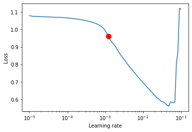
We see that this value of lr = 0.001 that we often used by default is actually often indeed a good choice.
del unet
unet = Unet(num_classes=3, learning_rate=1e-3)
logger = TensorBoardLogger("tb_logs", name="unet_triangle")
trainer = pl.Trainer(max_epochs=30, logger=logger)
trainer.fit(unet, train_dataloaders=train_loader, val_dataloaders=validation_loader)
GPU available: False, used: False
TPU available: False, using: 0 TPU cores
IPU available: False, using: 0 IPUs
Missing logger folder: tb_logs/unet_triangle

   | Name            | Type             | Params
------------------------------------------------------
0  | conv1           | Conv2d           | 160
1  | maxpool1        | MaxPool2d        | 0
2  | conv2           | Conv2d           | 4.6 K
3  | maxpool2        | MaxPool2d        | 0
4  | conv3           | Conv2d           | 18.5 K
5  | transpose_conv3 | ConvTranspose2d  | 8.2 K
6  | conv2_t         | Conv2d           | 18.5 K
7  | transpose_conv2 | ConvTranspose2d  | 2.1 K
8  | conv1_t         | Conv2d           | 4.6 K
9  | conv_final      | Conv2d           | 51
10 | loss            | CrossEntropyLoss | 0
------------------------------------------------------
56.7 K    Trainable params
0         Non-trainable params
56.7 K    Total params
0.227     Total estimated model params size (MB)
Validation sanity check: 0%| | 0/2 [00:00<?, ?it/s]
/Users/gw18g940/miniconda3/envs/CASImaging/lib/python3.9/site-packages/pytorch_lightning/trainer/data_loading.py:132: UserWarning: The dataloader, val_dataloader 0, does not have many workers which may be a bottleneck. Consider increasing the value of the `num_workers` argument` (try 4 which is the number of cpus on this machine) in the `DataLoader` init to improve performance.
  rank_zero_warn(
/Users/gw18g940/miniconda3/envs/CASImaging/lib/python3.9/site-packages/pytorch_lightning/trainer/data_loading.py:132: UserWarning: The dataloader, train_dataloader, does not have many workers which may be a bottleneck. Consider increasing the value of the `num_workers` argument` (try 4 which is the number of cpus on this machine) in the `DataLoader` init to improve performance.
  rank_zero_warn(
/Users/gw18g940/miniconda3/envs/CASImaging/lib/python3.9/site-packages/pytorch_lightning/trainer/data_loading.py:432: UserWarning: The number of training samples (40) is smaller than the logging interval Trainer(log_every_n_steps=50). Set a lower value for log_every_n_steps if you want to see logs for the training epoch.
  rank_zero_warn(
Epoch 11: 84%|████████▍ | 42/50 [00:10<00:02, 3.99it/s, loss=0.0591, v_num=0]
/Users/gw18g940/miniconda3/envs/CASImaging/lib/python3.9/site-packages/pytorch_lightning/trainer/trainer.py:688: UserWarning: Detected KeyboardInterrupt, attempting graceful shutdown...
  rank_zero_warn("Detected KeyboardInterrupt, attempting graceful shutdown...")
%load_ext tensorboard
%sstensorboard --logdir tb_logs
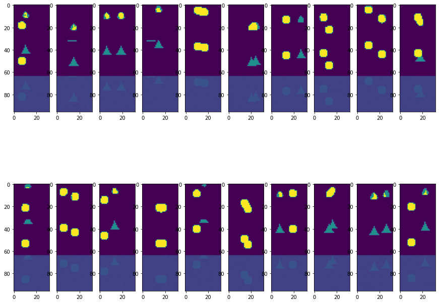
val_iter = iter(validation_loader)
test_batch, test_label = next(val_iter)
pred = unet(test_batch)
fig = plt.figure(figsize=(15,12))
spec = fig.add_gridspec(ncols=10, nrows=2)

ind=0
for row in range(2):
    for col in range(10):

        ax = fig.add_subplot(spec[row, col])
        ax.imshow(torch.cat((pred[ind].argmax(dim=0),test_label[ind], test_batch[ind,0])),vmin=0,vmax=2)
        ind +=1
Epoch 11: 84%|████████▍ | 42/50 [00:25<00:04, 1.65it/s, loss=0.0591, v_num=0]