7. Data augmentation
Contents
![]()
7. Data augmentation
Until now we have mostly played with synthetic data over which we have full control in terms of number of examples and content. Obviously that’s not the case in the “real world” where you might mostly encounter two problems: 1. not enough training data and 2. inference data that are not exactly matching data used for training. This is where data augmentation can be useful.
Imagine for example that you trained an algorithm to detect objects in an image that always have the same orientation. However now for your inference the “alignment” of your acquisition system is drifting and objects are slightly rotated. This will make impact the quality of your inference. The way to go around this is to artificially create variations in your training set in the hope to achieve a more general results.
We are using again our simple example with geometric figures. However now for inference we will rotate the images and see how it impacts the result.
# set path containing data folder or use default for Colab (/gdrive/My Drive)
local_folder = "../"
import urllib.request
urllib.request.urlretrieve('https://raw.githubusercontent.com/guiwitz/DLImaging/master/utils/check_colab.py', 'check_colab.py')
from check_colab import set_datapath
colab, datapath = set_datapath(local_folder)
Model and training
import torch
import torch.nn as nn
from torch.functional import F
import torch.optim as optim
from torch.utils.data import Dataset, DataLoader
from torch.utils.data import random_split

from skimage.draw import random_shapes
import matplotlib.pyplot as plt
import numpy as np
# define network
class Mynetwork(nn.Module):
    def __init__(self, input_size, num_categories):
        super(Mynetwork, self).__init__()

        # define e.g. layers here e.g.
        self.layer1 = nn.Linear(input_size, 100)
        self.layer2 = nn.Linear(100, 100)
        self.layer3 = nn.Linear(100, num_categories)

    def forward(self, x):

        # flatten the input
        x = x.flatten(start_dim=1)
        # define the sequence of operations in the network including e.g. activations
        x = F.relu(self.layer1(x))
        x = F.relu(self.layer2(x))
        x = self.layer3(x)

        return x

# define loss
criterion = nn.CrossEntropyLoss()

# define dataset
images = np.load(datapath.joinpath('data/triangle_circle.npy'))
labels = np.load(datapath.joinpath('data/triangle_circle_label.npy'))

class Tricircle(Dataset):
    def __init__(self, data, labels, transform=None):
        super(Tricircle, self).__init__()
        self.data = data
        self.labels = labels

    def __getitem__(self, index):

        x = self.data[index]
        x = torch.tensor(x/255, dtype=torch.float32)
        y = torch.tensor(self.labels[index])

        return x, y

    def __len__(self):

        return len(labels)

tridata = Tricircle(images, labels)

batch_size = 10
test_size = int(0.8 * len(tridata))
valid_size = len(tridata)-test_size
train_data, valid_data = random_split(tridata, [test_size, valid_size])

train_loader = DataLoader(train_data, batch_size=batch_size)
valid_loader = DataLoader(valid_data, batch_size=batch_size)
Train the model
num_classes = 2
model = Mynetwork(1024, num_classes)
optimizer = optim.Adam(model.parameters(), lr=0.001)
for epoch in range(2):
    print(f'epoch: {epoch}')
    # initialize accuracy
    running_accuracy = 0

    for t, data in enumerate(train_loader):

        # get batch
        mybatch, label = data

        # calculate predicted label and calculate loss
        pred = model(mybatch)
        loss = criterion(pred, label)

        # backpropagate the loss
        loss.backward()

        # do the optimization step
        optimizer.step()

        # set gradients to zero as PyTorch accumulates them otherwise
        optimizer.zero_grad()

        # calculate accuracy
        mean_accuracy = (torch.argmax(pred,dim=1) == label).sum()/batch_size
        running_accuracy+=mean_accuracy

        every_nth = 1000
        if t % every_nth == every_nth-1:
            print(f'accuracy: {running_accuracy/every_nth}')
            running_accuracy = 0.0

    # validation
    valid_accuracy=0
    for t, data in enumerate(valid_loader):

        # get batch
        mybatch, label = data

        # calculate predicted label
        pred = model(mybatch)
        # calculate accuracy
        mean_accuracy = (torch.argmax(pred,dim=1) == label).sum()/batch_size
        valid_accuracy+=mean_accuracy
    valid_accuracy = valid_accuracy/len(valid_loader)
    print(f'valid_accuracy: {valid_accuracy}')
epoch: 0
accuracy: 0.8467020392417908
accuracy: 0.9599016904830933
accuracy: 0.9839006662368774
accuracy: 0.990401029586792
valid_accuracy: 0.9943005442619324
epoch: 1
accuracy: 0.9947004318237305
accuracy: 0.9940004944801331
accuracy: 0.9943001866340637
accuracy: 0.997100293636322
valid_accuracy: 0.9976001977920532
Feeding rotated data
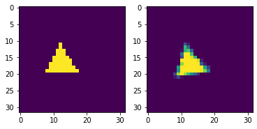
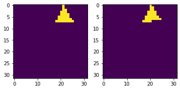
We can use the skimage.transform.rotate function to rotate some of our images.
import skimage.transform
image, _ = random_shapes((32,32),max_shapes=1, min_shapes=1, num_channels=1, shape='triangle',
                                min_size=8)
image = 255-image
image_rot = skimage.transform.rotate(image, 10, preserve_range=True)
fig, ax = plt.subplots(1,2)
ax[0].imshow(image)
ax[1].imshow(image_rot,)
<matplotlib.image.AxesImage at 0x142049340>
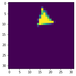
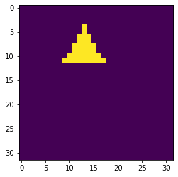
We adjust our generating function (in dlcourse.py and create one that rotates objects randomly:
from dlcourse import make_image_rot
image_rot = make_image_rot('triangle', np.random.randint(0,10))
plt.imshow(image_rot)
<matplotlib.image.AxesImage at 0x1422c1fd0>
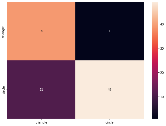
Let’s see how bad this is now:
from sklearn.metrics import confusion_matrix
import pandas as pd
import seaborn as sn
im_type = ['triangle', 'circle']
label_test = torch.randint(0,len(im_type),(100,))
mybatch_test = torch.stack([make_image_rot(im_type[x], np.random.randint(0,90)) for x in label_test])
pred = model(mybatch_test)
accuracy = (torch.argmax(pred,dim=1) == label_test).sum()/100
print(f'accuracy: {accuracy}')
accuracy: 0.7400000095367432
df_cm = pd.DataFrame(confusion_matrix(pred.argmax(dim=1), label_test), index = im_type,
                  columns = im_type)
plt.figure(figsize = (10,7))
sn.heatmap(df_cm, annot=True);
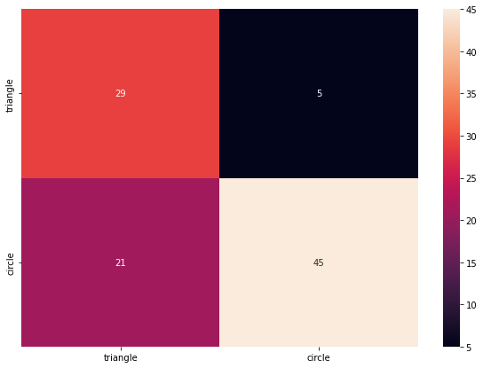
Obviously the problem only affects the triangle as the circle is rotationally invariant. So what can we do now? We can use data augmentation during training on our original un-rotated dataset. We will see later more general ways to do this but let’s for the moment just rotate our data using functions from torchvision.transforms:
import torchvision.transforms
rotation = torchvision.transforms.RandomRotation((0,40))
The nice thing with torchivision functions is that they accept batches by default. So we don’t have to rotate each image individually:
iter_loader = iter(train_loader)
single_batch = next(iter_loader)
single_batch, single_label = single_batch
rotated_single_batch = rotation(single_batch)
fig, ax = plt.subplots(1,2)
ax[0].imshow(single_batch[2,:,:])
ax[1].imshow(rotated_single_batch[2,:,:])
<matplotlib.image.AxesImage at 0x1445ac580>
model = Mynetwork(1024, len(im_type))
optimizer = optim.Adam(model.parameters(), lr=0.001)

for epoch in range(5):
    print(f'epoch: {epoch}')
    # initialize accuracy
    running_accuracy = 0

    for t, data in enumerate(train_loader):

        # get batch
        mybatch, label = data

        # !!!!!!!!!!!!!!!!!!!!!!!!!!!!!!!Augmentation!!!!!!!!!!!!!!!!!!!!!!!
        mybatch = rotation(mybatch)
        # !!!!!!!!!!!!!!!!!!!!!!!!!!!!!!!Augmentation!!!!!!!!!!!!!!!!!!!!!!!


        # calculate predicted label and calculate loss
        pred = model(mybatch)
        loss = criterion(pred, label)

        # backpropagate the loss
        loss.backward()

        # do the optimization step
        optimizer.step()

        # set gradients to zero as PyTorch accumulates them otherwise
        optimizer.zero_grad()

        # calculate accuracy
        mean_accuracy = (torch.argmax(pred,dim=1) == label).sum()/batch_size
        running_accuracy+=mean_accuracy

        every_nth = 1000
        if t % every_nth == every_nth-1:
            print(f'accuracy: {running_accuracy/every_nth}')
            running_accuracy = 0.0

    # validation
    valid_accuracy=0
    for t, data in enumerate(valid_loader):

        # get batch
        mybatch, label = data

        # calculate predicted label
        pred = model(mybatch)
        # calculate accuracy
        mean_accuracy = (torch.argmax(pred,dim=1) == label).sum()/batch_size
        valid_accuracy+=mean_accuracy
    valid_accuracy = valid_accuracy/len(valid_loader)
    print(f'valid_accuracy: {valid_accuracy}')
epoch: 0
accuracy: 0.7815008759498596
accuracy: 0.8975019454956055
accuracy: 0.9447022080421448
accuracy: 0.9625019431114197
valid_accuracy: 0.9551023840904236
epoch: 1
accuracy: 0.9750018119812012
accuracy: 0.9800010919570923
accuracy: 0.982601523399353
accuracy: 0.9864010214805603
valid_accuracy: 0.9808016419410706
epoch: 2
accuracy: 0.9904008507728577
accuracy: 0.9890009164810181
accuracy: 0.9899008274078369
accuracy: 0.9918006062507629
valid_accuracy: 0.9909006953239441
epoch: 3
accuracy: 0.9925005435943604
accuracy: 0.9920004606246948
accuracy: 0.9920007586479187
accuracy: 0.99470055103302
valid_accuracy: 0.9908008575439453
epoch: 4
accuracy: 0.9935004115104675
accuracy: 0.9932008385658264
accuracy: 0.9946005940437317
accuracy: 0.9941005706787109
valid_accuracy: 0.9944003224372864
We see that we might need more epochs to achieve good training. This is expected as we now have “more” training data.
Let’s see now if the network performs better on our directly generated rotated dataset:
pred = model(mybatch_test)
accuracy = (torch.argmax(pred,dim=1) == label_test).sum()/100
print(f'accuracy: {accuracy}')
accuracy: 0.8799999952316284
df_cm = pd.DataFrame(confusion_matrix(pred.argmax(dim=1), label_test), index = im_type,
                  columns = im_type)
plt.figure(figsize = (10,7))
sn.heatmap(df_cm, annot=True);
Combine augmentation
It is very common to integrate the augmentation step in the data loading process. One can specify what modification one wants to apply randomly to the loaded images. For example here we combined rotation, and rotation transformations. This is done by composing (using Compose) multiple augmentations in one module and passing it to the dataset. We see that we also integrate a stepf of conversion to tensor:
import torchvision.transforms

transforms = torchvision.transforms.Compose([
    torchvision.transforms.ToTensor(),
    torchvision.transforms.Resize((50,50)),
    torchvision.transforms.RandomRotation(20)
])
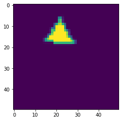
The expected input of transform is for example a Numpy array that should first be turned into a tensor, and then resized and rotated. We can see if that works with an image:
current_image = images[4,:,:]
plt.imshow(current_image)
<matplotlib.image.AxesImage at 0x144726940>
tfmed = transforms(current_image)
tfmed.size()
torch.Size([1, 50, 50])
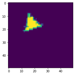
plt.imshow(tfmed[0,:,:])
<matplotlib.image.AxesImage at 0x1447a2580>
Now we can pass our transform object when creating the dataset.
class Tricircle(Dataset):
    def __init__(self, data, labels, transform=None):
        super(Tricircle, self).__init__()
        self.data = data
        self.labels = labels
        self.transform = transform

    def __getitem__(self, index):

        x = self.data[index]
        if self.transform:
            x = self.transform(x)
        y = torch.tensor(self.labels[index])

        return x, y

    def __len__(self):

        return len(labels)

tridata = Tricircle(images, labels)
tridata = Tricircle(images, labels, transforms)
plt.imshow(tridata[4][0][0,:,:])
<matplotlib.image.AxesImage at 0x144801820>