4. Simple neural net with PyTorch
Contents
![]()
4. Simple neural net with PyTorch
Neural networks can be programmed on different levels depending on how much one needs to customize either the architecture or the training pattern. When dealing with more complex NN we will use a higher-level package (Lightning, see Chapter 8) which will spare us some “manual” work. However, in order to understand all steps involved in designing a DL algorithm, we will first use basic PyTroch. In this notebook we will see howe we can design a NN while in the next notebook we will se how to train it.
# set path containing data folder or use default for Colab (/gdrive/My Drive)
local_folder = "../"
import urllib.request
urllib.request.urlretrieve('https://raw.githubusercontent.com/guiwitz/DLImaging/master/utils/check_colab.py', 'check_colab.py')
from check_colab import set_datapath
colab, datapath = set_datapath(local_folder)
Mounted at /gdrive
Layer from torch.nn
We will see in this notebook how to create a simple neural network for image classification using the most general mechanism in PyTorch which are modules. All module-related objects and functions are contained in torch.nn. As the name indicates, these modules are really modular in the sense that they are indpendent parts of networks that can be combined together. Mostly we will use single modules containing the multiple layers of our architecture, but we will also see examples where multiple modules are assembled.
A module is essentially an assemble of multiple other modules, and many of these are provided “pre-made” for us also available in torch.nn. For example in the simple network used here we will only use linear layers. Before we create an actual network let’s see how layers work:
from torch import nn
We creat now a linear layer that takes a vector of size 5 as input and ouptuts a vector of size 10:
lin_layer = nn.Linear(in_features=5, out_features=10)
This single layer already has parameters:
list(lin_layer.parameters())
[Parameter containing:
 tensor([[ 0.1772, -0.2716, -0.0833,  0.4179,  0.0139],
         [ 0.0236,  0.4233, -0.0906, -0.0667, -0.1381],
         [ 0.0183,  0.3365, -0.0383, -0.2230,  0.1193],
         [-0.1372, -0.1642,  0.0699,  0.2822, -0.0746],
         [-0.4264,  0.3427, -0.1457, -0.4305, -0.0769],
         [-0.1531, -0.0913,  0.1122, -0.1215, -0.0599],
         [-0.0187,  0.1361, -0.3873,  0.2272, -0.3454],
         [-0.3957, -0.3610, -0.0309,  0.3582,  0.2156],
         [ 0.3501,  0.2927, -0.1047,  0.4398, -0.1033],
         [ 0.2378,  0.0654, -0.3990, -0.2655,  0.1689]], requires_grad=True),
 Parameter containing:
 tensor([-0.2049, -0.0815,  0.4178, -0.3250,  0.3191, -0.3232, -0.1012,  0.0951,
          0.0309, -0.1550], requires_grad=True)]
We see that we have indeed a 5x10 matrix plus the bias term of size 10. When we later assemble multiple modules, we will see the same time of output but with many more parameters.
Passing an input
Our layer takes a vector as an input so let’s try to creat a vector of size 5 and pass it through the layer:
import numpy as np
myvector = np.random.randint(0,100,5)
myvector
array([93, 93, 44, 15, 90])
No we we pass it to lin_layer:
lin_layer(myvector)
---------------------------------------------------------------------------
TypeError                                 Traceback (most recent call last)
<ipython-input-7-6ef7c06b0ae8> in <module>()
----> 1 lin_layer(myvector)

/usr/local/lib/python3.7/dist-packages/torch/nn/modules/module.py in _call_impl(self, *input, **kwargs)
   1100         if not (self._backward_hooks or self._forward_hooks or self._forward_pre_hooks or _global_backward_hooks
   1101                 or _global_forward_hooks or _global_forward_pre_hooks):
-> 1102             return forward_call(*input, **kwargs)
   1103         # Do not call functions when jit is used
   1104         full_backward_hooks, non_full_backward_hooks = [], []

/usr/local/lib/python3.7/dist-packages/torch/nn/modules/linear.py in forward(self, input)
    101
    102     def forward(self, input: Tensor) -> Tensor:
--> 103         return F.linear(input, self.weight, self.bias)
    104
    105     def extra_repr(self) -> str:

/usr/local/lib/python3.7/dist-packages/torch/nn/functional.py in linear(input, weight, bias)
   1846     if has_torch_function_variadic(input, weight, bias):
   1847         return handle_torch_function(linear, (input, weight, bias), input, weight, bias=bias)
-> 1848     return torch._C._nn.linear(input, weight, bias)
   1849
   1850

TypeError: linear(): argument 'input' (position 1) must be Tensor, not numpy.ndarray
Of course we get an error, as the layer doesn’t expect a Numpy array but a PyTorch tensor! We can have a look at what PyTorch tensors are in the 03-Tensors notebook and come back here later.
Now we can turn our Numpy array into a tensor:
import torch
mytensor = torch.tensor(myvector)
mytensor
tensor([93, 93, 44, 15, 90])
lin_layer(mytensor)
---------------------------------------------------------------------------
RuntimeError                              Traceback (most recent call last)
<ipython-input-10-4eeffe384bb6> in <module>()
----> 1 lin_layer(mytensor)

/usr/local/lib/python3.7/dist-packages/torch/nn/modules/module.py in _call_impl(self, *input, **kwargs)
   1100         if not (self._backward_hooks or self._forward_hooks or self._forward_pre_hooks or _global_backward_hooks
   1101                 or _global_forward_hooks or _global_forward_pre_hooks):
-> 1102             return forward_call(*input, **kwargs)
   1103         # Do not call functions when jit is used
   1104         full_backward_hooks, non_full_backward_hooks = [], []

/usr/local/lib/python3.7/dist-packages/torch/nn/modules/linear.py in forward(self, input)
    101
    102     def forward(self, input: Tensor) -> Tensor:
--> 103         return F.linear(input, self.weight, self.bias)
    104
    105     def extra_repr(self) -> str:

/usr/local/lib/python3.7/dist-packages/torch/nn/functional.py in linear(input, weight, bias)
   1846     if has_torch_function_variadic(input, weight, bias):
   1847         return handle_torch_function(linear, (input, weight, bias), input, weight, bias=bias)
-> 1848     return torch._C._nn.linear(input, weight, bias)
   1849
   1850

RuntimeError: expected scalar type Long but found Float
Again an error! The error can be a bit misleading. The whole problem is that the weights in the layer are defined by default as float32. Hence the input should match this but we passed an 64 bits integer which creates a conflict. Let’s adjust the type of our tensor. We can either modify the tensor:
mytensor_float = mytensor.float()
mytensor_float
tensor([93., 93., 44., 15., 90.])
mytensor_float.dtype
torch.float32
or do it from the beginning when transforming our Numpy array by specifying the dtype explicitely:
mytensor_float = torch.tensor(myvector, dtype=torch.float32)
mytensor_float.dtype
torch.float32
Now we finally have the right object to path through our network:
output = lin_layer(mytensor_float)
output
tensor([ -5.1316,  24.0661,  39.1124, -27.7620, -27.2561, -25.3290, -33.9091,
        -46.8651,  52.5092,  21.6992], grad_fn=<AddBackward0>)
output.shape
torch.Size([10])
We see that the ouput has as expected as size of 10! Of course we can now add as many other layers as we want:
lin_layer2 = nn.Linear(10,3)
output = lin_layer2(output)
output.size()
torch.Size([3])
Activation
In addition to layers we will typically also need activation functions such as soft-max. Those are implemented as modules in torch.nn as well as functions in torch.functional which we use here:
import torch.nn.functional as F
Since we use the functional form, we can pass the output of the above linear layer directly to the activation function, here a ReLU:
lin_layer_activated = F.relu(output)
lin_layer_activated
tensor([4.6315, 0.0000, 0.0000], grad_fn=<ReluBackward0>)
Structure of a network
Now that we have seen how to create a layers and activation functions we can assemble them into a usable network structure. In PyTorch that structure is nn.Module a base class on top of which we can build our network. We can specify what parameters we want to pass when creating this object and we also have to define a single function, forward, which describes the network itself. Here’s an example:
class Mynetwork(nn.Module):
    def __init__(self, myparameter1, myparameter2):
        super(Mynetwork, self).__init__()

        # define e.g. layers here e.g.
        self.layer1 = nn.Linear(myparameter1, 5)
        self.layer2 = nn.Linear(5, myparameter2)

    def forward(self, x):

        # define the sequence of operations in the network including e.g. activations
        x = F.relu(self.layer1(x))
        x = self.layer2(x)

        return x
Above, we have defined a simple network that is defined by two parameters, myparameter1, myparameter2, and which is composed of two linear layers and ReLU unit. The differnt layers that we need are defined in __init__ as object parameters and then re-used in the network definition in the forward function. forward takes an input x (e.g. an image to classify), passes it through the network and outputs the result. Therefore in principle we could instantiate a model and use it like this:
mymodel = Mynetwork(9,3)
mymodel.forward(myinput)
However, nn.Module has a __call__ attribute that allows us to use the class as a function like this:
mymodel = Mynetwork(9,3)
mymodel(myinput)
This is actually how a module should be properly used in order to exploit all capabilities offered in PyTorch.
Let’s now try this out. We instantiate the model:
mymodel = Mynetwork(9,3)
Just like for the single linear layer before, we can have a look at all parameters:
list(mymodel.parameters())
[Parameter containing:
 tensor([[ 0.0483, -0.2518, -0.0089, -0.2222, -0.2226,  0.0678, -0.0117,  0.1295,
          -0.2652],
         [ 0.1032,  0.1222,  0.1620, -0.3203,  0.1332,  0.0745, -0.2601,  0.1932,
           0.0618],
         [ 0.3046,  0.0502,  0.1105,  0.0564, -0.1664, -0.0811,  0.1039,  0.0440,
           0.1922],
         [ 0.0937,  0.2563,  0.1606,  0.1038, -0.0500, -0.2383,  0.1778, -0.0871,
           0.1092],
         [-0.3318, -0.2407, -0.0272,  0.2387, -0.2174,  0.1162, -0.1696,  0.2630,
          -0.3218]], requires_grad=True), Parameter containing:
 tensor([ 0.1442,  0.3127, -0.3283,  0.2729, -0.2035], requires_grad=True), Parameter containing:
 tensor([[-0.3275, -0.3544, -0.0413,  0.1119, -0.1094],
         [-0.3663,  0.0042, -0.4315, -0.1468,  0.0556],
         [ 0.3742, -0.1017,  0.3442,  0.3889, -0.3229]], requires_grad=True), Parameter containing:
 tensor([ 0.1876,  0.3002, -0.2017], requires_grad=True)]
The output is the same, only now we see all parameters from all layers, not just a single one. We can also look at the modules contained in our network:
list(mymodel.modules())
[Mynetwork(
   (layer1): Linear(in_features=9, out_features=5, bias=True)
   (layer2): Linear(in_features=5, out_features=3, bias=True)
 ),
 Linear(in_features=9, out_features=5, bias=True),
 Linear(in_features=5, out_features=3, bias=True)]
We see some repeats because we see here modules at all levels. E.g. each linear layer is a module but our entire network is a module as well.
We can also just find all modules contained in our main module and recover its name and function:
for name, module in mymodel.named_children():
    print(f'name: {name} module: {module}')
name: layer1 module: Linear(in_features=9, out_features=5, bias=True)
name: layer2 module: Linear(in_features=5, out_features=3, bias=True)
We can also obtain a dictionary of all layers with their weights:
mymodel.state_dict()
OrderedDict([('layer1.weight',
              tensor([[ 0.0483, -0.2518, -0.0089, -0.2222, -0.2226,  0.0678, -0.0117,  0.1295,
                       -0.2652],
                      [ 0.1032,  0.1222,  0.1620, -0.3203,  0.1332,  0.0745, -0.2601,  0.1932,
                        0.0618],
                      [ 0.3046,  0.0502,  0.1105,  0.0564, -0.1664, -0.0811,  0.1039,  0.0440,
                        0.1922],
                      [ 0.0937,  0.2563,  0.1606,  0.1038, -0.0500, -0.2383,  0.1778, -0.0871,
                        0.1092],
                      [-0.3318, -0.2407, -0.0272,  0.2387, -0.2174,  0.1162, -0.1696,  0.2630,
                       -0.3218]])),
             ('layer1.bias',
              tensor([ 0.1442,  0.3127, -0.3283,  0.2729, -0.2035])),
             ('layer2.weight',
              tensor([[-0.3275, -0.3544, -0.0413,  0.1119, -0.1094],
                      [-0.3663,  0.0042, -0.4315, -0.1468,  0.0556],
                      [ 0.3742, -0.1017,  0.3442,  0.3889, -0.3229]])),
             ('layer2.bias', tensor([ 0.1876,  0.3002, -0.2017]))])
Finally we can pass an input through our network. It takes an input of size 9:
my_input = torch.randn((9,))
output = mymodel(my_input)
output
tensor([-0.3433, 0.0139, 0.0470], grad_fn=<AddBackward0>)
Batches
If we want to use batch processing, we can also pass batches of vectors thourgh the network instead of single vectors. PyTroch layers are designed to hanle this by default, so here for example if we want to use a batch of size 32 we can just use a 32 x 8 tensor. We create one directly with torch.randn here (we will learn more about batches in the chapter on training):
batch_tensor = torch.randn(32,9)
batch_tensor.shape
torch.Size([32, 9])
batch_output = mymodel(batch_tensor)
batch_output.shape
torch.Size([32, 3])
We see that the output is “batched” as well, so the network gracefully handlend this batch for us.
Passing an image as input
For the tests above, we simply used vectors. However our goal is to pass images to our network. As our network is linear and fully connected, we therefore need to pass a flattened (1D) version of our image. We have seen before that we can do that using the view method or flatten.
To test this, we first create a test image using the skimage.draw utility scikit-image which allows us to create random_shapes images:
from skimage.draw import random_shapes
import matplotlib.pyplot as plt
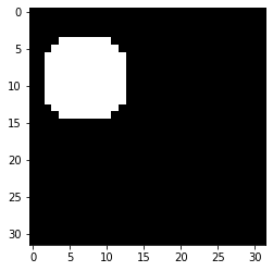
We create a 32x32 image of a circle. We have multiple options for the number of shapes, their size etc. to select from. We also invert the image (to have the object as foreground):
image_circle, _ = random_shapes((32,32),max_shapes=1, min_shapes=1, shape='circle',
                                num_channels=1, channel_axis=None, min_size=8, random_seed=2)
image_circle = 255-image_circle

image_tensor = torch.tensor(image_circle,dtype=torch.float32)
image_tensor.shape
torch.Size([32, 32])
plt.imshow(image_tensor, cmap='gray');
Now we flatten the image:
image_flat = image_tensor.view(-1)
image_flat.shape
torch.Size([1024])
We adjust our network input size:
mymodel = Mynetwork(1024,20)
output = mymodel(image_flat)
output
tensor([ 0.3483,  2.5287, -0.9607, -0.6729,  0.8906,  0.7305,  2.4549, -1.1527,
         1.9908, -1.9030, -1.1623, -0.4935,  1.7990,  1.3409, -0.3435, -1.2225,
        -1.7168,  2.4262,  0.0932, -1.4792], grad_fn=<AddBackward0>)
The operation of “flattening” can be done at different places. For example, instead of flattening the input, we can also flatten within our network definition:
class Mynetwork2(nn.Module):
    def __init__(self, myparameter1, myparameter2):
        super(Mynetwork2, self).__init__()

        # define e.g. layers here e.g.
        self.layer1 = nn.Linear(myparameter1, myparameter2)

    def forward(self, x):

        x = x.view(-1)
        # define the sequence of operations in the network including e.g. activations
        x = F.relu(self.layer1(x))

        return x
second_model = Mynetwork2(1024, 20)
output = second_model(image_tensor)
output
tensor([ 0.0000,  0.0000,  0.0000,  0.0000,  4.2747, 12.7591,  0.0000,  0.0000,
         3.2894,  3.1473,  0.0000,  0.0000,  0.0000,  0.0000,  0.0000,  0.0000,
        14.3413,  7.2331,  0.0000,  0.0000], grad_fn=<ReluBackward0>)
output.shape
torch.Size([20])
Saving and loading a model
Our next goal will be to train our network (see next chapter). At some point during or after training we will want to save both our model and its weights. This can be done in two ways.
Save full model
First, we can save the entire model so that it can be simply reloaded. This is practical when developing but can lead to problems when moving saved models between computers. First we save our model (create a models folder in your directory if needed):
torch.save(second_model, datapath.joinpath('models/simpleNN.pt'))
And reload it:
third_model = torch.load(datapath.joinpath('models/simpleNN.pt'))
third_model(image_tensor)
tensor([ 0.0000,  0.0000,  0.0000,  0.0000,  4.2747, 12.7591,  0.0000,  0.0000,
         3.2894,  3.1473,  0.0000,  0.0000,  0.0000,  0.0000,  0.0000,  0.0000,
        14.3413,  7.2331,  0.0000,  0.0000], grad_fn=<ReluBackward0>)
And we see that we obtain the same values as above, meaning that the parameters were indeed saved.
Saving the model state
Alternatively we can simply save all the parameters, which is a safer method. We simply recover them using state_dict:
torch.save(third_model.state_dict(),datapath.joinpath('models/simpleNN_state.pt'))
To reload the parameters we of course now have to first instantiate the model and “fill” it with those values using load_state_dict:
fourth_model = Mynetwork2(1024, 20)
params = torch.load(datapath.joinpath('models/simpleNN_state.pt'))
params
OrderedDict([('layer1.weight',
              tensor([[-6.5818e-03, -1.3050e-05, -2.1981e-02,  ...,  2.0436e-02,
                       -1.8892e-03, -2.1725e-02],
                      [ 2.0734e-02, -1.9473e-02, -2.8260e-02,  ...,  2.5199e-02,
                       -2.9951e-02,  8.9792e-03],
                      [-1.3109e-03,  1.3450e-02,  1.9928e-02,  ..., -5.7713e-03,
                        1.0590e-02, -1.9134e-02],
                      ...,
                      [ 1.6805e-02,  2.3167e-02,  3.1948e-03,  ..., -1.5454e-02,
                        1.3553e-02, -1.7430e-02],
                      [-2.3587e-02, -1.8857e-02,  9.4816e-03,  ...,  2.1235e-02,
                       -2.0854e-02, -2.8723e-02],
                      [ 2.1510e-03, -4.4486e-03, -1.7398e-02,  ..., -1.2099e-02,
                        1.0446e-02,  2.7855e-03]])),
             ('layer1.bias',
              tensor([ 0.0084,  0.0012,  0.0020,  0.0185,  0.0250, -0.0038,  0.0236, -0.0299,
                       0.0036,  0.0277, -0.0210, -0.0126, -0.0142, -0.0256, -0.0099,  0.0236,
                       0.0120, -0.0239,  0.0216, -0.0094]))])
fourth_model.load_state_dict(params)
<All keys matched successfully>
fourth_model(image_tensor)
tensor([ 0.0000,  0.0000,  0.0000,  0.0000,  4.2747, 12.7591,  0.0000,  0.0000,
         3.2894,  3.1473,  0.0000,  0.0000,  0.0000,  0.0000,  0.0000,  0.0000,
        14.3413,  7.2331,  0.0000,  0.0000], grad_fn=<ReluBackward0>)
Running on a GPU (run on Colab)
If you want to exploit the computational power of a GPU you have to take care of moving both the model and the data to it. First, find out if you have a GPU. You can test this for example by running this notebook on Colab:
torch.cuda.is_available()
True
If you have a GPU, you can define it as a device. If not you can fall back on CPU:
if torch.cuda.is_available():
    dev = torch.device("cuda")
else:
    dev = torch.device("cpu")
Now finally if you want to use it with a model you need to move the model to it. Let’s check where it currently sits:
second_model.to(dev)
Mynetwork2(
  (layer1): Linear(in_features=1024, out_features=20, bias=True)
)
list(second_model.parameters())
[Parameter containing:
 tensor([[-6.5818e-03, -1.3050e-05, -2.1981e-02,  ...,  2.0436e-02,
          -1.8892e-03, -2.1725e-02],
         [ 2.0734e-02, -1.9473e-02, -2.8260e-02,  ...,  2.5199e-02,
          -2.9951e-02,  8.9792e-03],
         [-1.3109e-03,  1.3450e-02,  1.9928e-02,  ..., -5.7713e-03,
           1.0590e-02, -1.9134e-02],
         ...,
         [ 1.6805e-02,  2.3167e-02,  3.1948e-03,  ..., -1.5454e-02,
           1.3553e-02, -1.7430e-02],
         [-2.3587e-02, -1.8857e-02,  9.4816e-03,  ...,  2.1235e-02,
          -2.0854e-02, -2.8723e-02],
         [ 2.1510e-03, -4.4486e-03, -1.7398e-02,  ..., -1.2099e-02,
           1.0446e-02,  2.7855e-03]], device='cuda:0', requires_grad=True),
 Parameter containing:
 tensor([ 0.0084,  0.0012,  0.0020,  0.0185,  0.0250, -0.0038,  0.0236, -0.0299,
          0.0036,  0.0277, -0.0210, -0.0126, -0.0142, -0.0256, -0.0099,  0.0236,
          0.0120, -0.0239,  0.0216, -0.0094], device='cuda:0',
        requires_grad=True)]
Now if we try to pass our current image through the network we get an error:
second_model(image_tensor)
---------------------------------------------------------------------------
RuntimeError                              Traceback (most recent call last)
<ipython-input-62-3dd5587f259c> in <module>()
----> 1 second_model(image_tensor)

/usr/local/lib/python3.7/dist-packages/torch/nn/modules/module.py in _call_impl(self, *input, **kwargs)
   1100         if not (self._backward_hooks or self._forward_hooks or self._forward_pre_hooks or _global_backward_hooks
   1101                 or _global_forward_hooks or _global_forward_pre_hooks):
-> 1102             return forward_call(*input, **kwargs)
   1103         # Do not call functions when jit is used
   1104         full_backward_hooks, non_full_backward_hooks = [], []

<ipython-input-44-4a29866e6538> in forward(self, x)
     10         x = x.view(-1)
     11         # define the sequence of operations in the network including e.g. activations
---> 12         x = F.relu(self.layer1(x))
     13
     14         return x

/usr/local/lib/python3.7/dist-packages/torch/nn/modules/module.py in _call_impl(self, *input, **kwargs)
   1100         if not (self._backward_hooks or self._forward_hooks or self._forward_pre_hooks or _global_backward_hooks
   1101                 or _global_forward_hooks or _global_forward_pre_hooks):
-> 1102             return forward_call(*input, **kwargs)
   1103         # Do not call functions when jit is used
   1104         full_backward_hooks, non_full_backward_hooks = [], []

/usr/local/lib/python3.7/dist-packages/torch/nn/modules/linear.py in forward(self, input)
    101
    102     def forward(self, input: Tensor) -> Tensor:
--> 103         return F.linear(input, self.weight, self.bias)
    104
    105     def extra_repr(self) -> str:

/usr/local/lib/python3.7/dist-packages/torch/nn/functional.py in linear(input, weight, bias)
   1846     if has_torch_function_variadic(input, weight, bias):
   1847         return handle_torch_function(linear, (input, weight, bias), input, weight, bias=bias)
-> 1848     return torch._C._nn.linear(input, weight, bias)
   1849
   1850

RuntimeError: Expected all tensors to be on the same device, but found at least two devices, cpu and cuda:0! (when checking argument for argument mat2 in method wrapper_mm)
The error message is quite explicit: you then need also to move the data, both for training and inference to the GPU:
image_tensor.to(dev)
tensor([[0., 0., 0.,  ..., 0., 0., 0.],
        [0., 0., 0.,  ..., 0., 0., 0.],
        [0., 0., 0.,  ..., 0., 0., 0.],
        ...,
        [0., 0., 0.,  ..., 0., 0., 0.],
        [0., 0., 0.,  ..., 0., 0., 0.],
        [0., 0., 0.,  ..., 0., 0., 0.]], device='cuda:0')
image_tensor = image_tensor.to(dev)
output = second_model(image_tensor)
output
tensor([ 0.0000,  0.0000,  0.0000,  0.0000,  4.2747, 12.7591,  0.0000,  0.0000,
         3.2894,  3.1473,  0.0000,  0.0000,  0.0000,  0.0000,  0.0000,  0.0000,
        14.3413,  7.2331,  0.0000,  0.0000], device='cuda:0',
       grad_fn=<ReluBackward0>)
The output sits on the GPU and is part of the gradient calcualtion, so if you want to further use it, you will have to pull it from the GPU and detach it from gradient calculation:
output.detach().cpu().numpy()
array([ 0.       ,  0.       ,  0.       ,  0.       ,  4.2747416,
       12.759116 ,  0.       ,  0.       ,  3.2893572,  3.1472843,
        0.       ,  0.       ,  0.       ,  0.       ,  0.       ,
        0.       , 14.341337 ,  7.2330832,  0.       ,  0.       ],
      dtype=float32)
Exercises
Create a network with 4 successive linear layers of size 20,40 and 100 and 2, and ReLU activation after the three first layers. It takes a 2D input.
With
skimage.ioimport the image in.../data/woody_baille.JPGInstantiate your model with the appropriate size
Run the image through the network and turn the output into a numpy array