Producing figures with multi-channel images#
The microplot module contains tools to create figures containing multi-channel images. It offers basic tools to turn 2D images into RGB images using specific color maps, combine multiple channels, create figures, adding labels and scale bars.
import matplotlib.pyplot as plt
import numpy as np
import skimage.io

from microfilm import microplot
Basic plotting with microshow#
The microshow function should be seen as an “enhanced” version of the Matplotlib imshow function which specifically deals with representing multi-channel images. In this first section, we see how to use that function and apply basic customizations.
Load images#
The microshow can take as input a Numpy array or a list of images (more on input format in the Image inputs section). Here we load a multi-dimensional image as a Numpy array, and also extract each channel as an individual stack:
image = skimage.io.imread('../demodata/coli_nucl_ori_ter.tif')
image.shape
(3, 30, 220, 169)
This image has 30 time points and 3 channels. We take now just the time t=10:
multi_channel = image[:,10,:,:]
multi_channel.shape
(3, 220, 169)
We also isolate each channel:
image1 = multi_channel[0]
image2 = multi_channel[1]
image3 = multi_channel[2]
print(f'image shape: {image1.shape}')
print(f'image type: {image1.dtype}')
image shape: (220, 169)
image type: uint16
Creating a default plot#
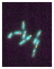
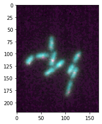
We can use the microshow function to plot our multi-channel image. If no options are passed, by default the image will be represented using the the color-blind friendly magenta-cyan-yellow color combination:
microim = microplot.microshow(images=multi_channel)
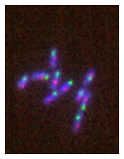
However we can easily adjust the color maps or lookup tables with the cmaps option. Here you can use any Matplotlib colormap as well as any map from the cmap library which collects maps from several sources (as a legacy you can still use pure_red, pure_green, pure_blue, pure_cyan, pure_yellow and pure_magenta but those will eventually be removed):
microim = microplot.microshow(images=multi_channel, cmaps=['blue', 'red', 'green'])
2D Image inputs#
As shown above, we can use a simple Numpy array as input. The dimension ordering is expected to be CXY i.e. Channel/X/Y. You can use np.swapaxis or np.moveaxis for example to change the dimensions to match this requirement. If you pass a Numpy array, all channels are plotted and therefore you need to provide the corresponding number of color maps (if not using default RGB).
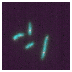
Alternatively you can also pass lists of images. This is useful if for example you don’t want to plot all channels of a Numpy array. For example you could use the following to only plot two out of the three channels:
microim = microplot.microshow(images=[multi_channel[1], multi_channel[2]])
3D image inputs#
You also have the possibility to represent 3D data as a projection (to reperesent 3D data as volumes, we recommend using napari. In this case, you need to provide either a Numpy array of dimensions CZXY or a list of 3D images of dimensions ZXY. As microshow cannot know if you want to plot multiple channels or a volume (both arrays have three dimensions), if you want to plot a volume you have two choices. You can pass an additional key-word volume_proj where you have the choices min, max, mean or you can use the volshow function which is identical to microshow but sets volume_proj='max' by default. As an example we load here the following dataset, composed of 20 time points, 11 slices and 2 channesl:
image3d = skimage.io.imread('../microfilm/dataset/tests/test_folders/coli_nucl_ori_3d.tif')
image3d.shape
(2, 20, 11, 200, 200)
microplot.microshow(image3d[:,0,:,:,:], volume_proj='mean');
microplot.volshow(image3d[:,0,:,:,:]);
Options at creation#
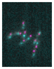
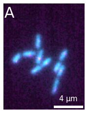
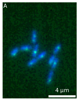
When we create the image, we have a large set of options that we can use to adjust the plot. For example, in addition to selecting specific color maps with cmaps, we can also choose a color projection type, add a scale bar and a label etc.:
microim = microplot.microshow(images=[image1, image2], cmaps=['cyan','magenta'], proj_type='sum',
                              unit='um', scalebar_unit_per_pix=0.065, scalebar_size_in_units=4,
                              scalebar_font_size=15, scalebar_thickness=0.02,
                              label_text='A', label_font_size=30);
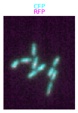
We can also add the channel labels as titles:
microim = microplot.microshow(images=[image1, image2], cmaps=['cyan','magenta'],
                              channel_label_show=True, channel_label_size=0.05,
                              channel_names=['CFP', 'RFP'])
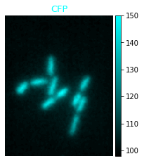
Colorbar#
If you plot an image with a single channel, you can add a colorbar to your plot. The limits of intensities correspond to the limits usde during plotting and specified e.g. with the limits and rescale_type options:
micro_colorbar = microplot.microshow(images=[image1], cmaps=['cyan'],
                              channel_label_show=True, channel_label_size=0.05,
                              channel_names=['CFP'], show_colorbar=True)
Microimage object#
When calling microshow, actually a Microimage instance is returned, which gives access to both specific functions of that instance as well as to the underlying Matplotlib objects.
Microimage methods#
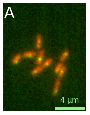
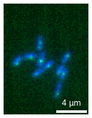
In the examples above, we always passed all inputs at time of figure creation. Alternatively to this, one can also first create a Microimage object and then use its attached methods such as add_label and add_scalebar to modify the plot. This can make the code slightly more readable:
microim = microplot.microshow(images=[image1, image2], cmaps=['red', 'green'])
microim.add_scalebar(unit='um', scalebar_unit_per_pix=0.065, scalebar_size_in_units=4,
                     scalebar_color='lightgreen', scalebar_font_size=15)
microim.add_label(label_text='A', label_font_size=30);
Relation to Matplotlib#
In the same spirit as e.g. the seaborn library, the microplot module stays very close to Matplotlib, so that you can integrate the image plots into larger figures. There are two ways in which microplot and Matplotlib are related.
First, the Microimage object gives access to the axis of the figure which allows you to use any Matplotlib customization on your plot. For example, you can turn the axes back on:
microim = microplot.microshow(images=[image1, image2])
microim.ax.set_axis_on()
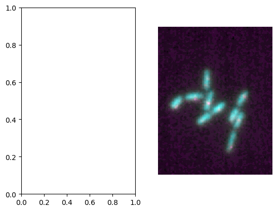
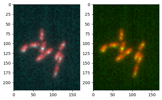
Second, you can integrate and microplot in existing Matplotlib figures again by using the axis. For that you can for example first create a subplot and re-use the axis reference as parameter in microshow to integrate the plot in that figure:
fig, ax = plt.subplots(1,2)
microim = microplot.microshow(images=[image1, image2], ax=ax[1]);
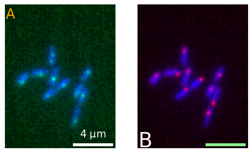
We can then of course use these approaches together. For example, we can first create Matplotlib subplots, add the micrplot in that figure, and then add labels to each microplot:
fig, ax = plt.subplots(1,2)
micro1 = microplot.microshow(images=[image1, image2], cmaps=['blue', 'green'],
                              scalebar_unit_per_pix=0.065, scalebar_size_in_units=4, unit='um',
                    scalebar_font_size=15, scalebar_color='white', ax=ax[0]);
micro2 = microplot.microshow(images=[image1, image3], cmaps=['blue', 'red'],
                              scalebar_unit_per_pix=0.065, scalebar_size_in_units=4, unit='um',
                    scalebar_font_size=None, scalebar_color='lightgreen', ax=ax[1])#, scalebar_kwargs={'scale_loc':'top'});

micro1.add_label('A', label_location='upper left', label_font_size=20, label_color='orange')
micro2.add_label('B', label_location='lower left', label_font_size=30);
Copying figures#
Matplotlib makes it impossible to re-use a given plot in multiple figures. Once you have created a microplot with annotations you might however want to re-use it in another larger figure. The microimage object allows you to do that since it stores all the relevant information and can easily be recreated. For example let’s create a plot:
micro1 = microplot.microshow(images=[image1, image2], cmaps=['blue', 'green'],
                             scalebar_unit_per_pix=0.065, scalebar_size_in_units=4, unit='um',
                             scalebar_font_size=15, scalebar_color='white');
And now we create a new figure with plt.subplots() and we can add our plot from above to it using the update method:
fig2, ax2 = plt.subplots()
newmicro1 = micro1.update(ax=ax2, copy=True)
newmicro1.add_label('A');
As an alternative to creating subplots yourself, you can also create a Micropanel object and add to it a series of microimages. Find more information in this section.
Lower level functions#
When calling microshow, several internal functions are used, e.g. to rescale the image intensity, combined multiple colormaps etc. You also have access to these functions individually from the colorify module.
from microfilm import colorify
Convert image to display with chosen colormap#
Using the colorify_by_name function, you can turn a single 2D array into a RGB image with a given colormap. You can use any colormap from Matplotlib and from cmap:
image2
array([[ 98,  99, 100, ..., 100, 100, 100],
       [ 99,  99,  99, ..., 100,  99,  99],
       [ 99,  98,  99, ...,  99,  99,  99],
       ...,
       [100, 100, 100, ...,  99,  99,  99],
       [100,  99,  99, ...,  99,  99,  99],
       [ 99,  99,  99, ...,  99, 100, 100]], dtype=uint16)
im_green, cmap, min_max = colorify.colorify_by_name(
    image2, cmap_name='green', flip_map=False, rescale_type='min_max')
plt.imshow(im_green);
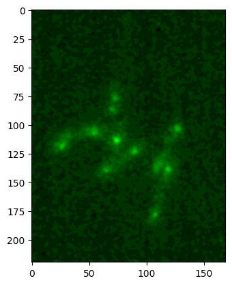
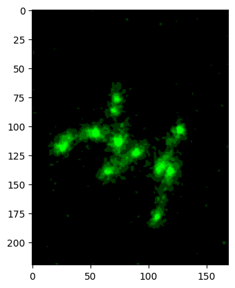
By default the image intensity is rescaled using the min-max values. This is often sub-optimal (e.g. if single pixels are way out of the distribution) and you can specify another rescaling. For example you can explicitly provide lower and upper limits:
im_green, cmap, min_max = colorify.colorify_by_name(
    image2, cmap_name='green', flip_map=False, rescale_type='limits',
                                       limits=[100,105])
plt.imshow(im_green);
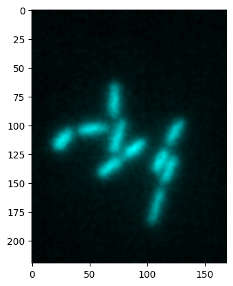
colormap hex#
Alternatively to the keyword based map, you can also use a hexadecimal encoding of a color to create an colormap ranging from black to that color. This gives more flexibility:
heximage, cmap, min_max = colorify.colorify_by_hex(image1, cmap_hex='#00ffff')
plt.imshow(heximage);
Combining images#
After having converted images to a given colormap, you can combine them into a single image with overlayed colors. Currently you can use a maximum projection (default) or a sum to replicate the Fiji behavior. You can simply use the combine_image function for that:
im1_mapped, _, _ = colorify.colorify_by_name(image1, cmap_name='red')
im2_mapped, _, _ = colorify.colorify_by_hex(image2, cmap_hex='#00ffff')


im1_mapped_b, _, _ = colorify.colorify_by_name(image1, cmap_name='red')
im2_mapped_b, _, _ = colorify.colorify_by_name(image2, cmap_name='green')

combined = colorify.combine_image([im1_mapped, im2_mapped])
combined_b = colorify.combine_image([im1_mapped_b, im2_mapped_b])

fig, ax = plt.subplots(1,2)
ax[0].imshow(combined)
ax[1].imshow(combined_b);
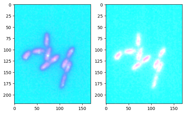
In the plots below, we compare the two available projections, maximum and sum. The difference is mostly visible when using colormaps that have large overlap, e.g. here with summer and cool. With pure_green and pure_red there would for example be no visual difference.
im1_mapped_b, _, _ = colorify.colorify_by_name(image1, cmap_name='cool')
im2_mapped_b, _, _ = colorify.colorify_by_name(image2, cmap_name='summer')

combined = colorify.combine_image([im1_mapped_b, im2_mapped_b], proj_type='max')
combined_b = colorify.combine_image([im1_mapped_b, im2_mapped_b], proj_type='sum')

fig, ax = plt.subplots(1,2, figsize=(7,7))
ax[0].imshow(combined)
ax[1].imshow(combined_b);
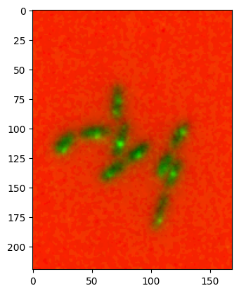
Direct conversion#
To save some steps you can also directly use a list of images and of colormaps to create a combined image:
converted, _, _, _ = colorify.multichannel_to_rgb(
    images=[image1, image2], cmaps=['red', 'green'], flip_map=[True, False])
plt.imshow(converted);
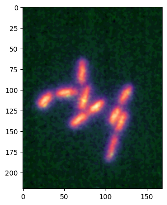
Most of these functions also work directly with Numpy arrays:
converted, _, _, _ = colorify.multichannel_to_rgb(images=[image1, image2], cmaps=['magma', 'green'])
plt.imshow(converted);
The scalebar#
We have seen above, that you could add a scalebar to the image. These scalebars are added via the matplotlib-scalebar package.
The only parameters needed for the scalebar are the unit that you use e.g. um, the size per pixel unit_per_pixel e.g. 0.5um/pixels, and the size of the scale bar scalebar_size_in_units in your unit e.g. 40um. In addition you can pass options like scalebar_color or scalebar_font_size to adjust the rendering. Note that you can pass a dictionary scalebar_kwargs with all possible options avaialble in the original ScaleBar object:
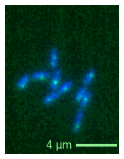
microim = microplot.microshow(images=[image1, image2], cmaps=['blue', 'green'],
                              unit='um', scalebar_unit_per_pix=0.065, scalebar_size_in_units=4,
                              scalebar_color='lightgreen', scalebar_font_size=15,
                              scalebar_kwargs={'scale_loc':'left'});
Export#
As the figure is simply a Matplotlib figure, you can just use the regular savefig function (and use this trick to avoid white space around the plot). You could access it via microim.fig.savefig but we also directly wrap it here in the microim object:
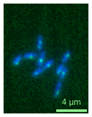
microim = microplot.microshow(images=[image1, image2], cmaps=['blue', 'green'],
                              unit='um', scalebar_unit_per_pix=0.065, scalebar_size_in_units=4,
                              scalebar_color='lightgreen', scalebar_font_size=15);
microim.savefig('single.png', bbox_inches = 'tight', pad_inches = 0, dpi=600)
And for more complex plots, you can just use the regular figure creation:
fig, ax = plt.subplots(1,2)
micro1 = microplot.microshow(images=[image1, image2], cmaps=['green', 'blue'],
                             scalebar_unit_per_pix=0.065, scalebar_size_in_units=4, unit='um',
                             scalebar_font_size=15, scalebar_color='white', ax=ax[0]);
micro2 = microplot.microshow(images=[image1, image2], cmaps=['red', 'blue'],
                             scalebar_unit_per_pix=0.065, scalebar_size_in_units=4, unit='um',
                             scalebar_font_size=None, scalebar_color='lightgreen', ax=ax[1]);

micro1.add_label('A', label_location='upper left', label_font_size=20, label_color='orange')
micro2.add_label('B', label_location='lower left', label_font_size=30);
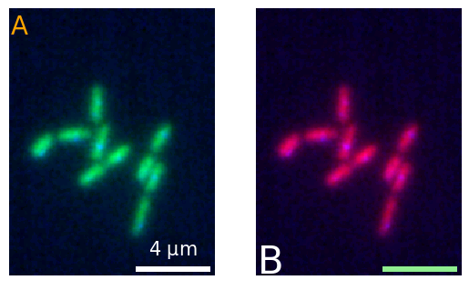
fig.savefig('figure.png', bbox_inches = 'tight', pad_inches = 0, dpi=600)
fig.savefig('figure.pdf', bbox_inches = 'tight', pad_inches = 0, dpi=600)