.ipynb .pdf

Binder

Contents

7. Creating a pipeline

In the previous chapter we created a procedure to isolate nuclei from images. Very often the goal is to repeat the exercise on multiple images in order to compare different conditions. Here we are going to see how to package our pipeline into a function, how to apply it to multiple images and how to plot the result for comparison.

import numpy as np
import pandas as pd
import matplotlib.pyplot as plt
import skimage
import skimage.io
import skimage.morphology
from scipy import ndimage as ndi

Creating an image processing function

We have seen previously how to define a function. It needs the def descriptor, a name and inputs. What we are doing here is just copying all the lines that we used for our pipeline in the last chapter into this function. At the moment the only input is the path to a given file to analyze. We also try to document what the function does, what its input/output are etc.

def my_pipeline(image_path):
    """
    This function extracts information about nuclei found in the third channel of an image
    loaded at the given path
    
    Parameters
    ----------
    image_path: str
        path to image
        
    Returns
    -------
    my_table: pandas dataframe
        dataframe with label, area, mean_intensity and extent information for each nucleus
    
    """
    
    image_stack = skimage.io.imread(image_path)
    
    image_nuclei = image_stack[:,:,2]#blue channel in RGB
    image_signal = image_stack[:,:,1]#green channel in RGB

    # filter image
    image_nuclei = skimage.filters.median(image_nuclei, skimage.morphology.disk(5))

    # create mask and clean-up
    mask_nuclei = image_nuclei > skimage.filters.threshold_otsu(image_nuclei)
    mask_nuclei = skimage.morphology.binary_closing(mask_nuclei, footprint=skimage.morphology.disk(5))
    mask_nuclei = ndi.binary_fill_holes(mask_nuclei, skimage.morphology.disk(5))
    
    # label image
    my_labels = skimage.morphology.label(mask_nuclei)

    # measure
    my_regions = skimage.measure.regionprops_table(my_labels, image_signal, properties=('label','area', 'mean_intensity'))
    
    plt.subplots(figsize=(10,10))
    plt.imshow(mask_nuclei)
    plt.show()
    
    my_table = pd.DataFrame(my_regions)
    
    return my_table
                
                

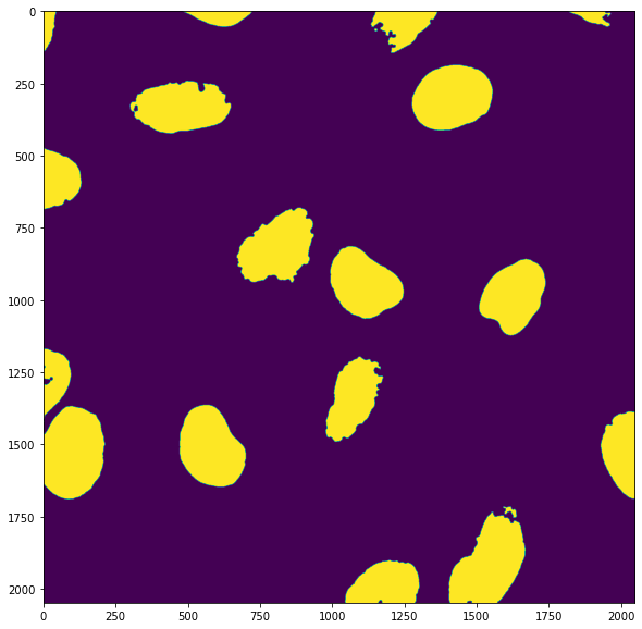
We can now test our function with a single image:

table = my_pipeline('https://github.com/guiwitz/PyImageCourse_beginner/raw/master/images/46658_784_B12_1.tif')

table

	label	area	mean_intensity
0	1	4221	79.265103
1	2	8386	65.997734
2	3	18258	70.261091
3	4	4043	63.026713
4	5	73	47.438356
5	6	49056	53.714510
6	7	45671	53.807099
7	8	20537	70.453912
8	9	46853	66.137729
9	10	43277	41.412552
10	11	40768	58.675039
11	12	15090	44.198144
12	13	35404	74.771551
13	14	47642	41.701902
14	15	54978	35.904107
15	16	26774	53.077874
16	17	4	112.000000
17	18	812	102.986453
18	19	54298	56.110207
19	20	29638	66.283791

Adjusting the function behavior

We have recovered the same result as previously and can analyze again our data as we did before. The mask is also plotted by default when calling the function. This is helpful to test the function and verify that nothing went dramatically wrong but we probably don’t want to see this image if we analyze hundreds of images. What we can do is leave the user the choice to see it or not. Let’s adjust our function to do that: we add an additional optional parameter do_plotting which is simply a boolean (True/False). If True, plotting is happening, if False it’s not.

def my_pipeline(image_path, do_plotting=False):
    """
    This function extracts information about nuclei found in the third channel of an image
    loaded at the given path
    
    Parameters
    ----------
    image_path: str
        path to image
    do_plotting: bool
        show segmentation or not
        
    Returns
    -------
    my_table: pandas dataframe
        dataframe with label, area, mean_intensity and extent information for each nucleus
    
    """
    
    image_stack = skimage.io.imread(image_path)
    
    image_nuclei = image_stack[:,:,2]#blue channel in RGB
    image_signal = image_stack[:,:,1]#green channel in RGB

    # filter image
    image_nuclei = skimage.filters.median(image_nuclei, skimage.morphology.disk(5))

    # create mask and clean-up
    mask_nuclei = image_nuclei > skimage.filters.threshold_otsu(image_nuclei)
    mask_nuclei = skimage.morphology.binary_closing(mask_nuclei, selem=skimage.morphology.disk(5))
    mask_nuclei = ndi.binary_fill_holes(mask_nuclei, skimage.morphology.disk(5))
    
    # label image
    my_labels = skimage.morphology.label(mask_nuclei)

    # measure
    my_regions = skimage.measure.regionprops_table(my_labels, image_signal, properties=('label','area', 'mean_intensity'))
    
    if do_plotting:
        plt.subplots(figsize=(10,10))
        plt.imshow(mask_nuclei)
        plt.show()
    
    my_table = pd.DataFrame(my_regions)
    
    return my_table
                
                

You see that we added an ìf statment in our code. This is the place where we control for plotting or not. To learn more about it, visit the next notebook!

table = my_pipeline('https://github.com/guiwitz/PyImageCourse_beginner/raw/master/images/46658_784_B12_1.tif')

Now indeed our function doesn’t produce any output if we don’t explicitly ask for it.

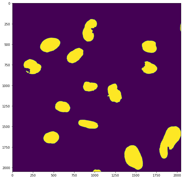
Analyzing multiple images

The point of creating an image processing pipeline was to be able to easily analyze multiple images. We can do that now by using a simple for loop. First we create a list of files we want to analyze and that we can see here and here.

files_to_analyze = [
    'https://github.com/guiwitz/PyImageCourse_beginner/raw/master/images/46658_784_B12_1.tif',
    'https://github.com/guiwitz/PyImageCourse_beginner/raw/master/images/27897_273_C8_2.tif'
]

Now we create a for loop that will go through this list of files and analyze each of them with our function. To learn more about for loops visit the next chapter on Logical Flow. Before the loop, we create an empty list that is going to be filled with the output of the function. We also add to the output DataFrame a column with the filename that we can recover by splitting the address files_to_analyze[0].split('/')[-1]. Note that the split function is a method of string objects that allows to split string where we find a certain character (here /):

all_tables = []
for file in files_to_analyze:
    
    #use the function
    new_table = my_pipeline(file)
    
    #add image index
    new_table['filename'] = file.split('/')[-1]
    
    #append the result to the list
    all_tables.append(new_table)
    

Finally we can concatenate our results into a single table. For this we use a Pandas function called concat which just glues two DataFrames together:

complete_info = pd.concat(all_tables)
complete_info

	label	area	mean_intensity	filename
0	1	4221	79.265103	46658_784_B12_1.tif
1	2	8386	65.997734	46658_784_B12_1.tif
2	3	18258	70.261091	46658_784_B12_1.tif
3	4	4043	63.026713	46658_784_B12_1.tif
4	5	73	47.438356	46658_784_B12_1.tif
5	6	49056	53.714510	46658_784_B12_1.tif
6	7	45671	53.807099	46658_784_B12_1.tif
7	8	20537	70.453912	46658_784_B12_1.tif
8	9	46853	66.137729	46658_784_B12_1.tif
9	10	43277	41.412552	46658_784_B12_1.tif
10	11	40768	58.675039	46658_784_B12_1.tif
11	12	15090	44.198144	46658_784_B12_1.tif
12	13	35404	74.771551	46658_784_B12_1.tif
13	14	47642	41.701902	46658_784_B12_1.tif
14	15	54978	35.904107	46658_784_B12_1.tif
15	16	26774	53.077874	46658_784_B12_1.tif
16	17	4	112.000000	46658_784_B12_1.tif
17	18	812	102.986453	46658_784_B12_1.tif
18	19	54298	56.110207	46658_784_B12_1.tif
19	20	29638	66.283791	46658_784_B12_1.tif
0	1	31346	91.784279	27897_273_C8_2.tif
1	2	1022	118.964775	27897_273_C8_2.tif
2	3	32149	108.144048	27897_273_C8_2.tif
3	4	21866	87.044407	27897_273_C8_2.tif
4	5	25406	82.585177	27897_273_C8_2.tif
5	6	26270	93.764675	27897_273_C8_2.tif
6	7	19557	101.465102	27897_273_C8_2.tif
7	8	2	20.500000	27897_273_C8_2.tif
8	9	16367	70.146331	27897_273_C8_2.tif
9	10	28357	77.683218	27897_273_C8_2.tif
10	11	19552	73.210158	27897_273_C8_2.tif
11	12	19288	75.883036	27897_273_C8_2.tif
12	13	58364	87.722003	27897_273_C8_2.tif
13	14	22228	105.550837	27897_273_C8_2.tif
14	15	49020	73.625255	27897_273_C8_2.tif
15	16	2009	68.762071	27897_273_C8_2.tif

We can then check if there’s any difference in intensity in the nucleus between the two images:

plt.hist(all_tables[0]['mean_intensity'], bins = np.arange(0,150,10), color = 'red')
plt.hist(all_tables[1]['mean_intensity'], bins = np.arange(0,150,10), alpha = 0.5, color = 'blue')
plt.show()

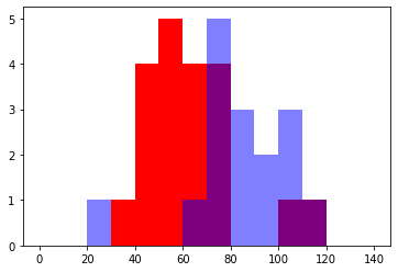
Of course our actual goal is not just to measure the intensity within the nucleus but to compare the intensity inside and on the edge of the nuclei. This is demonstrated in the Demo notebooks.

previous

6. Region properties

next

8. Loops and conditions