1. Python and notebook basics¶

In this first chapter, we will cover the very essentials of Python and notebooks such as creating a variable, importing packages, using functions, seeing how variables behave in the notebook etc. We will see more details on some of these topics, but this very short introduction will then allow us to quickly dive into more applied and image processing specific topics without having to go through a full Python introduction.

Variables¶

Like we would do in mathematics when we define variables in equations such as \(x=3\), we can do the same in all programming languages. Python has one of the simplest syntax for this, i.e. exactly as we would do it naturally. Let’s define a variable in the next cell:

a = 3

As long as we don’t execute the cell using Shift+Enter or the play button in the menu, the above cell is purely text. We can close our Jupyter session and then re-start it and this line of text will still be there. However other parts of the notebook are not “aware” that this variable has been defined and so we can’t re-use anywhere else. For example if we type a again and execute the cell, we get an error:

---------------------------------------------------------------------------
NameError                                 Traceback (most recent call last)
/var/folders/mk/632_7fgs4v374qc935pvf9v00000gn/T/ipykernel_18079/2167009006.py in <cell line: 1>()
----> 1 a

NameError: name 'a' is not defined

So we actually need to execute the cell so that Python reads that line and executes the command. Here it’s a very simple command that just says that the value of the variable a is three. So let’s go back to the cell that defined a and now execute it (click in the cell and hit Shift+Enter). Now this variable is stored in the computing memory of the computer and we can re-use it anywhere in the notebook (but only in this notebook)!

We can again just type a

We see that now we get an output with the value three. Most variables display an output when they are not involved in an operation. For example the line a=3 didn’t have an output.

Now we can define other variables in a new cell. Note that we can put as many lines of commands as we want in a single cell. Each command just need to be on a new line.

b = 5
c = 2

As variables are defined for the entire notebook we can combine information that comes from multiple cells. Here we do some basic mathematics:

a + b

Here we only see the output. We can’t re-use that ouput for further calculations as we didn’t define a new variable to contain it. Here we do it:

d = a + b

d is now a new variable. It is purely numerical and not a mathematical formula as the above cell could make you believe. For example if we change the value of a:

a = 100

and check the value of d:

it has not change. We would have to rerun the operation and assign it again to d for it to update:

d = a + b
d

We will see many other types of variables during the course. Some are just other types of data, for example we can define a text variable by using quotes ' ' around a given text:

my_text = 'This is my text'
my_text

'This is my text'

Others can contain multiple elements like lists:

my_list = [3, 8, 5, 9]
my_list

[3, 8, 5, 9]

but more on these data structures later…

Functions¶

We have seen that we could define variables and do some basic operations with them. If we want to go beyond simple arithmetic we need more complex functions that can operate on variables. Imagine for example that we need a function \(f(x, a, b) = a * x + b\). For this we can use and define functions. Here’s how we can define the previous function:

def my_fun(x, a, b):
    out = a * x + b
    return out

We see a series of Python rules to define a function:

we use the word def to signal that we are creating a function
we pick a function name, here my_fun
we open the parenthesis and put all our variables x, a, b in there, just like when we do mathematics
we do some operation inside the function. Inside the function is signal with the indentation: everything that belong inside the function (there could be many more lines) is shifted by a single tab or three space to the right
we use the word return to tell what is the output of the function, here the variable out

We can now use this function as if we were doing mathematics: we pick a a value for the three parameters e.g. \(f(3, 2, 5)\)

my_fun(3, 2, 5)

Note that some functions are defined by default in Python. For example if I define a variable which is a string:

my_text = 'This is my text'

I can count the number of characters in this text using the len() function which comes from base Python:

len(my_text)

The len function has not been manually defined within a def statement, it simply exist by default in the Python language.

Variables as objects¶

In the Python world, variables are not “just” variables, they are actually more complex objects. So for example our variable my_text does indeed contain the text This is my text but it contains also additional features. The way to access those features is to use the dot notation my_text.some_feature. There are two types of featues:

functions, called here methods, that do some computation or modify the variable itself
properties, that contain information about the variable

For example the object my_text has a function attached to it that allows us to put all letters to lower case:

my_text

'This is my text'

my_text.lower()

'this is my text'

If we define a complex number:

a = 3 + 5j

then we can access the property real that gives us only the real part of the number:

a.real

3.0

Note that when we use a method (function) we need to use the parenthesis, just like for regular functions, while for properties we don’t.

Packages¶

In the examples above, we either defined a function ourselves or used one generally accessible in base Python but there is a third solution: external packages. These packages are collections of functions used in a specific domain that are made available to everyone via specialized online repositories. For example we will be using in this course a package called scikit-image that implements a large number of functions for image processing. For example if we want to filter an image stored in a variable im_in with a median filter, we can then just use the median() function of scikit-image and apply it to an image im_out = median(im_in). The question is now: how do we access these functions?

Importing functions¶

The answer is that we have to import the functions we want to use in a given notebook from a package to be able to use them. First the package needs to be installed. One of the most popular place where to find such packages is the PyPi repository. We can install packages from there using the following command either in a terminal or directly in the notebook. For example for scikit-image:

pip install scikit-image

Requirement already satisfied: scikit-image in /Users/gw18g940/mambaforge/envs/improc_beginner/lib/python3.9/site-packages (0.19.2)
Requirement already satisfied: networkx>=2.2 in /Users/gw18g940/mambaforge/envs/improc_beginner/lib/python3.9/site-packages (from scikit-image) (2.7.1)
Requirement already satisfied: tifffile>=2019.7.26 in /Users/gw18g940/mambaforge/envs/improc_beginner/lib/python3.9/site-packages (from scikit-image) (2022.2.9)
Requirement already satisfied: PyWavelets>=1.1.1 in /Users/gw18g940/mambaforge/envs/improc_beginner/lib/python3.9/site-packages (from scikit-image) (1.2.0)
Requirement already satisfied: pillow!=7.1.0,!=7.1.1,!=8.3.0,>=6.1.0 in /Users/gw18g940/mambaforge/envs/improc_beginner/lib/python3.9/site-packages (from scikit-image) (9.0.1)
Requirement already satisfied: scipy>=1.4.1 in /Users/gw18g940/mambaforge/envs/improc_beginner/lib/python3.9/site-packages (from scikit-image) (1.8.0)
Requirement already satisfied: packaging>=20.0 in /Users/gw18g940/mambaforge/envs/improc_beginner/lib/python3.9/site-packages (from scikit-image) (21.3)
Requirement already satisfied: imageio>=2.4.1 in /Users/gw18g940/mambaforge/envs/improc_beginner/lib/python3.9/site-packages (from scikit-image) (2.16.1)
Requirement already satisfied: numpy>=1.17.0 in /Users/gw18g940/mambaforge/envs/improc_beginner/lib/python3.9/site-packages (from scikit-image) (1.22.2)
Requirement already satisfied: pyparsing!=3.0.5,>=2.0.2 in /Users/gw18g940/mambaforge/envs/improc_beginner/lib/python3.9/site-packages (from packaging>=20.0->scikit-image) (3.0.7)
Note: you may need to restart the kernel to use updated packages.

Once installed we can import the packakge in a notebook in the following way (note that the name of the package is scikit-image, but in code we use an abbreviated name skimage):

import skimage

The import is valid for the entire notebook, we don’t need that line in each cell.

Now that we have imported the package we can access all function that we define in it using a dot notation skimage.myfun. Most packages are organized into submodules and in that case to access functions of a submodule we use skimage.my_submodule.myfun.

To come back to the previous example: the median filtering function is in the filters submodule that we could now use as:

im_out = skimage.filters.median(im_in)

We cannot execute this command as the variables im_in and im_out are not yet defined.

Note that there are multiple ways to import packages. For example we could give another name to the package, using the as statement:

import skimage as sk

Nowe if we want to use the median function in the filters sumodule we would write:

im_out = sk.filters.median(im_in)

We can also import only a certain submodule using:

from skimage import filters

Now we have to write:

im_out = filters.median(im_in)

Finally, we can import a single function like this:

from skimage.filters import median

and now we have to write:

im_out = median(im_in)

Structures¶

As mentioned above we cannot execute those various lines like im_out = median(im_in) because the image variable im_in is not yet defined. This variable should be an image, i.e. it cannot be a single number like in a=3 but an entire grid of values, each value being one pixel. We therefore need a specific variable type that can contain such a structure.

We have already seen that we can define different types of variables. Single numbers:

a = 3

Text:

b = 'my text'

or even lists of numbers:

c = [6,2,8,9]

This last type of variable is called a list in Python and is one of the structures that is available in Python. If we think of an image that has multiple lines and columns of pixels, we could now imagine that we can represent it as a list of lists, each single list being e.g. one row pf pixels. For example a 3 x 3 image could be:

my_image = [[4,8,7], [6,4,3], [5,3,7]]
my_image

[[4, 8, 7], [6, 4, 3], [5, 3, 7]]

While in principle we could use a list for this, computations on such objects would be very slow. For example if we wanted to do background correction and subtract a given value from our image, effectively we would have to go through each element of our list (each pixel) one by one and sequentially remove the background from each pixel. If the background is 3 we would have therefore to compute:

4-3
8-3
7-3
6-3

etc. Since operations are done sequentially this would be very slow as we couldn’t exploit the fact that most computers have multiple processors. Also it would be tedious to write such an operation.

To fix this, most scientific areas that use lists of numbers of some kind (time-series, images, measurements etc.) resort to an external package called Numpy which offers a computationally efficient list called an array.

To make this clearer we now import an image in our notebook to see such a structure. We will use a function from the scikit-image package to do this import. That function called imread is located in the submodule called io. Remember that we can then access this function with skimage.io.imread(). Just like we previously defined a function \(f(x, a, b)\) that took inputs \(x, a, b\), this imread() function also needs an input. Here it is just the location of the image, and that location can either be the path to the file on our computer or a url of an online place where the image is stored. Here we use an image that can be found at https://github.com/guiwitz/PyImageCourse_beginner/raw/master/images/19838_1252_F8_1.tif. As you can see it is a tif file. This address that we are using as an input should be formatted as text:

my_address = 'https://github.com/guiwitz/PyImageCourse_beginner/raw/master/images/19838_1252_F8_1.tif'

Now we can call our function:

skimage.io.imread(my_address)

array([[[42, 48,  0],
        [45, 41,  0],
        [47, 21,  0],
        ...,
        [78, 16,  1],
        [57, 14,  0],
        [53,  7,  0]],

       [[42, 57,  0],
        [37, 40,  0],
        [38, 30,  0],
        ...,
        [97,  7,  0],
        [67, 12,  0],
        [57,  9,  1]],

       [[42, 55,  0],
        [44, 40,  0],
        [31, 29,  0],
        ...,
        [79,  0,  0],
        [67,  1,  0],
        [61,  1,  0]],

       ...,

       [[ 0,  0,  0],
        [ 0,  0,  0],
        [ 0,  0,  0],
        ...,
        [65, 37,  0],
        [54, 37,  0],
        [47, 49,  0]],

       [[ 0,  0,  0],
        [ 0,  0,  0],
        [ 0,  0,  0],
        ...,
        [75, 41,  0],
        [59, 44,  0],
        [54, 74,  0]],

       [[ 0,  0,  0],
        [ 0,  0,  0],
        [ 0,  0,  0],
        ...,
        [82, 51,  0],
        [62, 48,  0],
        [57, 69,  0]]], dtype=uint8)

We see here an output which is what is returned by our function. It is as expected a list of numbers, and not all numbers are shown because the list is too long. We see that we also have [] to specify rows, columns etc. The main difference compared to our list of lists that we defined previously is the array indication at the very beginning of the list of numbers. This array indication tells us that we are dealing with a Numpy array, this alternative type of list of lists that will allow us to do efficient computations.

Plotting¶

We will see a few ways to represent data during the course. Here we just want to have a quick look at the image we just imported. For plotting we will use yet another external library called Matplotlib. That library is extensively used in the Python world and offers extensive choices of plots. We will mainly use one function from the library to display images: imshow. Again, to access that function, we first need to import the package. Here we need a specific submodule:

import matplotlib.pyplot as plt

Now we can use the plt.imshow() function. There are many options for plot, but we can use that function already by just passing an array as an input. First we need to assign the imported array to a variable:

import skimage.io

image = skimage.io.imread(my_address)

plt.imshow(image);

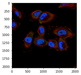
We see that we are dealing with a multi-channel image and can already distinguish cell nuclei (blue) and cytoplasm (red).

Image processing with Python for beginners

1. Python and notebook basics

Contents